Functions, loops, and if/else statements
Getting started
Remember everything in a line after the # sign is comments that will not be run. Look in these comments for practice exercises for the tutorial, which will be marked #Practice
Always begin by setting the working directory (the folder on your computer where R will read and write data files) I like to start by asking R for the current working directory to remind me of the correct formatting
getwd()Now set the desired working directory. Your code will look different from mine here.
setwd("/Users/leedietterich/Dropbox/STRI R course/Lecture 20200506 LD")Practice: set your own working directory
Read in a data table. This is an abbreviated dataset from Dietterich et al. 2017 Ecological Applications. In brief, I collected leaves, roots, and soils from many individuals of five plant species growing throughout a site contaminated with zinc, lead, and cadmium. I sought to understand the relationships between soil metal concentrations, root colonization by arbuscular mycorrhizal fungi (AMF), and leaf metal concentrations. The provided dataset gives AMF colonization (percent of root length colonized), and pollutant concentrations of leaves and soils in mg/kg.
mydata <- read.csv("Dietterich et al 2017 data for R course.csv")
#Use the structure command to make sure R is interpreting the data frame correctly
str(mydata)
#Convert the Species column to a factor
mydata$Species <- as.factor(mydata$Species)
#Convert the AMF column from proportion to percent
mydata$AMF <- mydata$AMF*100
Let’s make a table of the averages ± standard errors of AMF colonization and all of the metal concentrations for each species.
Recall how the mean function works, and experiment with how it handles NA values (we’ll see why soon). Make two vectors which are identical except that one has a couple NA values, and test the mean function on both of them.
x.test <- 1:10
x.test.with.nas <- c(1:3, NA, NA, 4:8, NA, 9, 10)
mean(x.test)
## [1] 5.5mean(x.test.with.nas)## [1] NAHere are two ways of removing NA values before calculating the mean. First, using the na.rm argument within the mean function
mean(x.test.with.nas, na.rm=T)## [1] 5.5Second, using the na.omit function
na.omit(x.test.with.nas)## [1] 1 2 3 4 5 6 7 8 9 10
## attr(,"na.action")
## [1] 4 5 11
## attr(,"class")
## [1] "omit"mean(na.omit(x.test.with.nas))## [1] 5.5Writing functions
The aggregate function is very useful for doing calculations on multiple treatment groups at once. As an example, we’ll calculate the average AMF colonization of each species in the experiment.
agg.amf <- with(mydata, aggregate(AMF, by=list(Species), FUN=mean))
agg.amf
## Group.1 x
## 1 AA NA
## 2 AP NA
## 3 DF NA
## 4 ES NA
## 5 MP NAThis returns all NA values because the mean function’s default does not handle NAs the way we want. We’ll need to write a function that calculates averages but omits NA values.
First, an introduction to function notation.
xplustwo <- function(x) x+2For simple functions like this, the curly brackets are optional, but you will need them for more complicated functions so I will use them consistently.
xcubed <- function(x) {
  x^3
}
Let’s test our new functions.
xplustwo(5)## [1] 7xcubed(8)## [1] 512x.test## [1] 1 2 3 4 5 6 7 8 9 10xplustwo(x.test)## [1] 3 4 5 6 7 8 9 10 11 12xcubed(x.test)## [1] 1 8 27 64 125 216 343 512 729 1000Now, the function we want to calculate the average of all NA values in a vector x.
avg <- function(x) {
  mean(na.omit(x))
}
While we’re at it, let’s write a similar function to calculate standard error. Recall that the standard error of a vector is the standard deviation divided by the square root of the sample size.
se <- function(x) {
  sd(na.omit(x))/sqrt(length(na.omit(x)))
}
For more complicated functions, it can be helpful to define variables inside the function. Here’s another way of writing the se function above.
se2 <- function(x) {
    y <- na.omit(x)
    return(sd(y)/sqrt(length(y)))
}
Let’s test these functions on the same vector, with and without NA values, and make sure they give the same answer.
x.test <- 1:10
x.test.with.nas <- c(1:3, NA, NA, 4:8, NA, 9, 10)

mean(x.test)
## [1] 5.5avg(x.test)## [1] 5.5mean(x.test.with.nas)## [1] NAavg(x.test.with.nas)## [1] 5.5sd(x.test)/sqrt(length(x.test))## [1] 0.9574271se(x.test)## [1] 0.9574271se2(x.test)## [1] 0.9574271sd(x.test.with.nas)/sqrt(length(x.test.with.nas))## [1] NAse(x.test.with.nas)## [1] 0.9574271se2(x.test.with.nas)## [1] 0.9574271Practice: write a function takes the average of a vector of numbers without using the mean function. Check that it works. Bonus if it works on vectors with NA values too!
Practice: write a function that takes the log+1 transform of a vector of numbers. That is, for each number in the vector, add one and then take the logarithm, base 10. Check that it works. Bonus if it works on vectors with NA values too!
Let’s get back to the table we started in line 31. We’ll start with just AMF colonization as an example.
agg.amf2 <- with(mydata, aggregate(AMF, by=list(Species), FUN=avg))
agg.amf2
## Group.1 x
## 1 AA 9.166572
## 2 AP 2.428819
## 3 DF 5.964999
## 4 ES 13.400351
## 5 MP 1.080950#Notice that aggregate doesn't preserve column names. Let's correct that.
names(agg.amf2) <- c("Species", "Average AMF colonization")
agg.amf2## Species Average AMF colonization
## 1 AA 9.166572
## 2 AP 2.428819
## 3 DF 5.964999
## 4 ES 13.400351
## 5 MP 1.080950We can make our table much more efficiently by using aggregate on many columns at once.
#Look at the column names of mydata to see which column numbers we want to aggregate
names(mydata)
## [1] "Sample.id" "Species" "AMF" "Cd.leaf" "Pb.leaf" "Zn.leaf"
## [7] "Cd.soil" "Pb.soil" "Zn.soil"#Run the aggregate
agg.avg <- with(mydata, aggregate(mydata[,3:9], by=list(Species), FUN=avg))
#Look at the results
agg.avg## Group.1 AMF Cd.leaf Pb.leaf Zn.leaf Cd.soil Pb.soil Zn.soil
## 1 AA 9.166572 16.550551 62.883543 1217.2924 51.28371 650.0625 5140.286
## 2 AP 2.428819 9.552666 23.731515 1195.8129 90.49262 1027.4266 6923.761
## 3 DF 5.964999 4.116137 10.794596 376.2118 43.73006 1186.7936 2942.489
## 4 ES 13.400351 34.452875 41.123450 1533.0363 70.74253 475.6594 6650.177
## 5 MP 1.080950 52.731918 7.612877 6450.6295 441.23633 2380.3515 35435.358#Here only the first column needs to be renamed
names(agg.avg)[1] <- "Species"
agg.avg## Species AMF Cd.leaf Pb.leaf Zn.leaf Cd.soil Pb.soil Zn.soil
## 1 AA 9.166572 16.550551 62.883543 1217.2924 51.28371 650.0625 5140.286
## 2 AP 2.428819 9.552666 23.731515 1195.8129 90.49262 1027.4266 6923.761
## 3 DF 5.964999 4.116137 10.794596 376.2118 43.73006 1186.7936 2942.489
## 4 ES 13.400351 34.452875 41.123450 1533.0363 70.74253 475.6594 6650.177
## 5 MP 1.080950 52.731918 7.612877 6450.6295 441.23633 2380.3515 35435.358Generate standard errors by the same technique
agg.se <- with(mydata, aggregate(mydata[,3:9], by=list(Species), FUN=se))
names(agg.se)[1] <- "Species"
agg.se
Let’s round all of the entries in both of these dataframes to three significant figures to make the table look pretty.
?roundTest the signif command on one column
round.test1 <- signif(agg.avg$AMF, 3)
round.test1
## [1] 9.17 2.43 5.96 13.40 1.08#Can signif handle multiple columns at once?
round.test2 <- signif(agg.avg[,2:8], 3)
round.test2## AMF Cd.leaf Pb.leaf Zn.leaf Cd.soil Pb.soil Zn.soil
## 1 9.17 16.60 62.90 1220 51.3 650 5140
## 2 2.43 9.55 23.70 1200 90.5 1030 6920
## 3 5.96 4.12 10.80 376 43.7 1190 2940
## 4 13.40 34.50 41.10 1530 70.7 476 6650
## 5 1.08 52.70 7.61 6450 441.0 2380 35400#Yes it can!Make a table of all of our pretty averages
round.avg <- with(agg.avg, cbind(Species, signif(agg.avg[,2:8], 3)))
round.avg
## Species AMF Cd.leaf Pb.leaf Zn.leaf Cd.soil Pb.soil Zn.soil
## 1 AA 9.17 16.60 62.90 1220 51.3 650 5140
## 2 AP 2.43 9.55 23.70 1200 90.5 1030 6920
## 3 DF 5.96 4.12 10.80 376 43.7 1190 2940
## 4 ES 13.40 34.50 41.10 1530 70.7 476 6650
## 5 MP 1.08 52.70 7.61 6450 441.0 2380 35400Make a table of pretty SEs by the same technique
round.se <- with(agg.avg, cbind(Species, signif(agg.se[,2:8], 3)))
round.se
## Species AMF Cd.leaf Pb.leaf Zn.leaf Cd.soil Pb.soil Zn.soil
## 1 AA 1.460 2.130 11.900 208.0 13.10 162.0 1090
## 2 AP 0.717 0.770 2.500 133.0 12.20 102.0 1080
## 3 DF 2.070 0.315 1.800 51.1 9.96 162.0 414
## 4 ES 2.550 4.250 5.950 137.0 13.20 87.7 1260
## 5 MP 0.534 5.760 0.564 591.0 71.50 359.0 6020To finish our table, we want each cell of columns 2 through 8 to display our rounded average, the character ±, and then our rounded SE. We will use a technique called a “for loop” to do this one cell at a time.
Loops
Here is a simple for loop to demonstrate the technique.
for(ii in 1:5){
  print(ii^2)
}
## [1] 1
## [1] 4
## [1] 9
## [1] 16
## [1] 25It can be convenient to embed loops inside functions. As an example, we’ll calculate the sum of squared deviations from a sample average. That is, for a vector x, we will find the average, calculate the difference of each element of x from that average, square that difference, and sum those differences for all elements of x.
sum.of.squares <- function(x){
    #Make an empty vector of the correct length where we will fill in our values
    sq.diffs <- rep(NA, length(x))
    for(ii in 1:length(x)){
        #Define each element of sq.diffs as the squared difference we want
        sq.diffs[ii] <- (x[ii]-mean(x))^2
        }
    #Return the sum of the entries in sq.diffs
    return(sum(sq.diffs))
}
Test this function
x.test## [1] 1 2 3 4 5 6 7 8 9 10sum.of.squares(x.test)## [1] 82.5Note that this function can also be done without a for loop.
sum((x.test-mean(x.test))^2)## [1] 82.5Let’s get back to our table. We’ll start with an empty destination table again as we did with the sum of squares function, but we’ll leave the Species column as it is because it doesn’t need anything new done to it.
The following code defines variables ii and jj and uses them to cycle through the rows and columns, respectively, of mytable. Then it defines entry [ii,jj] of mytable by concatenating the corresponding values of round.avg and round.se, separated by the character string " ± ".
mytable <- round.avg
for(ii in 1:5){
    for(jj in 2:8){
        mytable[ii,jj] <- paste(round.avg[ii,jj], round.se[ii,jj], sep=" ± ")
    }
}
mytable
## Species AMF Cd.leaf Pb.leaf Zn.leaf Cd.soil
## 1 AA 9.17 ± 1.46 16.6 ± 2.13 62.9 ± 11.9 1220 ± 208 51.3 ± 13.1
## 2 AP 2.43 ± 0.717 9.55 ± 0.77 23.7 ± 2.5 1200 ± 133 90.5 ± 12.2
## 3 DF 5.96 ± 2.07 4.12 ± 0.315 10.8 ± 1.8 376 ± 51.1 43.7 ± 9.96
## 4 ES 13.4 ± 2.55 34.5 ± 4.25 41.1 ± 5.95 1530 ± 137 70.7 ± 13.2
## 5 MP 1.08 ± 0.534 52.7 ± 5.76 7.61 ± 0.564 6450 ± 591 441 ± 71.5
## Pb.soil Zn.soil
## 1 650 ± 162 5140 ± 1090
## 2 1030 ± 102 6920 ± 1080
## 3 1190 ± 162 2940 ± 414
## 4 476 ± 87.7 6650 ± 1260
## 5 2380 ± 359 35400 ± 6020Save mytable as a csv.
write.csv(mytable, file="My pretty table.csv")For some reason when I open this resulting file in Excel, I get the symbol  before each ±, which seems to be a problem of text encoding between R and Excel but easy to fix in find/change. Interestingly when I read it back into R it displays correctly again:
mypretty <- read.csv(file="My pretty table.csv")
mypretty
## X Species AMF Cd.leaf Pb.leaf Zn.leaf Cd.soil
## 1 1 AA 9.17 ± 1.46 16.6 ± 2.13 62.9 ± 11.9 1220 ± 208 51.3 ± 13.1
## 2 2 AP 2.43 ± 0.717 9.55 ± 0.77 23.7 ± 2.5 1200 ± 133 90.5 ± 12.2
## 3 3 DF 5.96 ± 2.07 4.12 ± 0.315 10.8 ± 1.8 376 ± 51.1 43.7 ± 9.96
## 4 4 ES 13.4 ± 2.55 34.5 ± 4.25 41.1 ± 5.95 1530 ± 137 70.7 ± 13.2
## 5 5 MP 1.08 ± 0.534 52.7 ± 5.76 7.61 ± 0.564 6450 ± 591 441 ± 71.5
## Pb.soil Zn.soil
## 1 650 ± 162 5140 ± 1090
## 2 1030 ± 102 6920 ± 1080
## 3 1190 ± 162 2940 ± 414
## 4 476 ± 87.7 6650 ± 1260
## 5 2380 ± 359 35400 ± 6020Practice with indexing: recreate mytable but with the columns in the following order: Cd.soil, Cd.leaf, Pb.soil, Pb.leaf, Zn.soil, Zn.leaf, AMF
Practice (more complicated): make a table in the style of mytable, but instead of presenting mean ± SE, present the lower and upper bounds of an approximate 95% confidence interval: mean ± 2*SD.
Hint: there are many ways to organize this. I suggest using aggregate with perhaps one or more homemade functions to calculate the numbers you want to put in the table, and then using a loop as above to arrange the numbers correctly into the table.
Note: if you’re actually trying to publish a 95% confidence interval you will want to use a more statistically rigorous version!
Moving toward if/else statements
Suppose we are interested in the relationships between plant and soil metal concentrations for each species: for instance, is the amount of Zn in the soil under species AA related to the amount of Zn in the leaves of AA? Let’s make a table where, for each plant species and each metal studied, we report whether the relationship between plant and soil metal concentrations is positive, negative, or not significant.
Statistical background: linear regression
This technique asks whether there is a significant linear relationship between two continuous variables. For example, let’s look at Zn in species AP
For the rows of mydata in which Species is AP, run a linear model of Zn.leaf as predicted by Zn.soil
AP.Zn.model <- with(mydata[mydata$Species=="AP",], lm(Zn.leaf~Zn.soil))
#View model summary
summary(AP.Zn.model)
##
## Call:
## lm(formula = Zn.leaf ~ Zn.soil)
##
## Residuals:
## Min 1Q Median 3Q Max
## -950.6 -199.1 -104.3 187.1 1182.0
##
## Coefficients:
## Estimate Std. Error t value Pr(>|t|)
## (Intercept) 443.86803 116.61543 3.806 0.000705 ***
## Zn.soil 0.08760 0.01264 6.931 1.55e-07 ***
## ---
## Signif. codes: 0 '***' 0.001 '**' 0.01 '*' 0.05 '.' 0.1 ' ' 1
##
## Residual standard error: 417 on 28 degrees of freedom
## (8 observations deleted due to missingness)
## Multiple R-squared: 0.6318, Adjusted R-squared: 0.6186
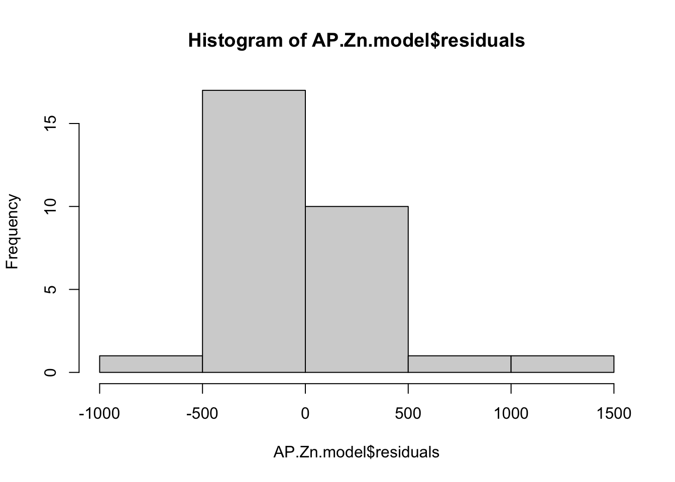
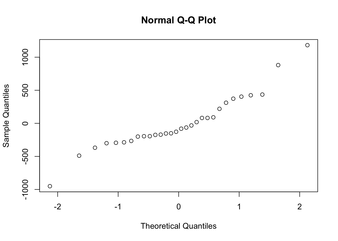
## F-statistic: 48.04 on 1 and 28 DF, p-value: 1.555e-07Regression assumes residuals are normally distributed - here are two ways of checking that. A histogram of the residuals should approximate a bell curve
hist(AP.Zn.model$residuals)
A normal quantile-quantile plot should approximate a 1:1 line.
qqnorm(AP.Zn.model$residuals)
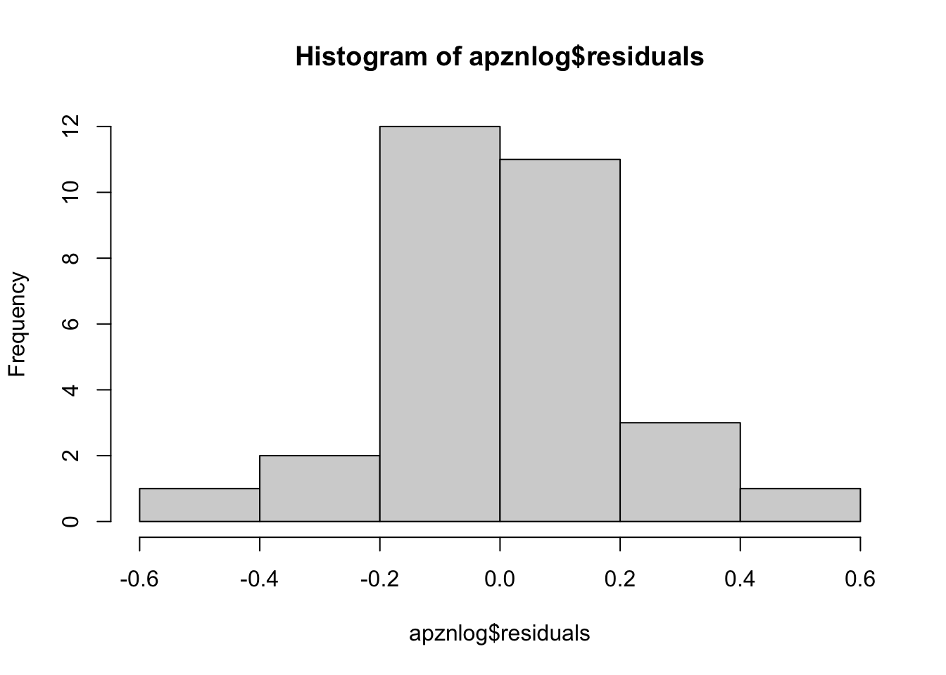
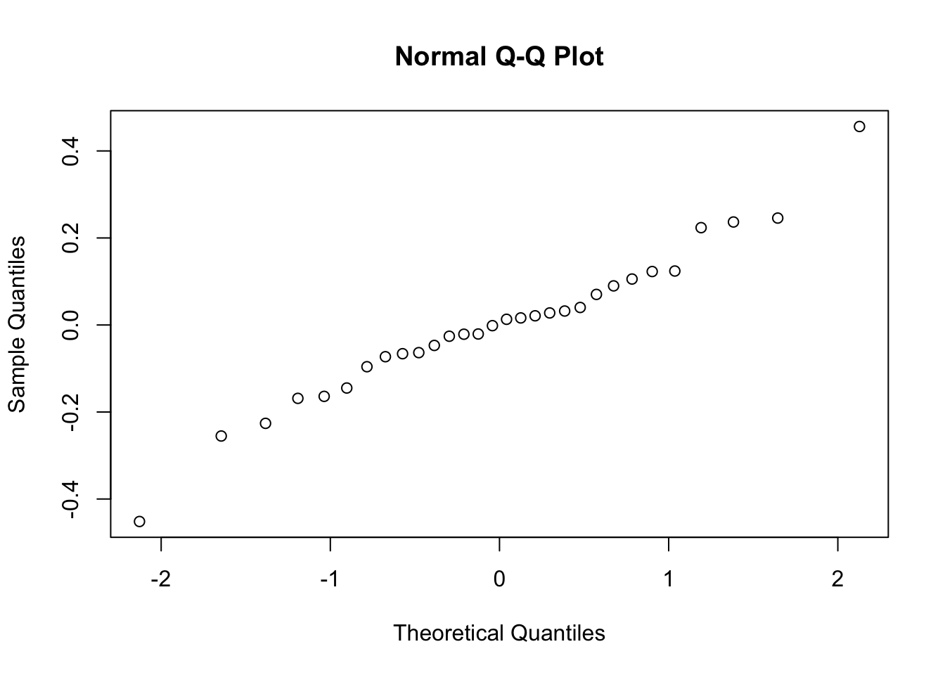
Does log-transformation help?
apznlog <- with(mydata[mydata$Species=="AP",], lm(log10(Zn.leaf)~log10(Zn.soil)))
summary(apznlog)
##
## Call:
## lm(formula = log10(Zn.leaf) ~ log10(Zn.soil))
##
## Residuals:
## Min 1Q Median 3Q Max
## -0.45167 -0.07118 0.00576 0.08498 0.45617
##
## Coefficients:
## Estimate Std. Error t value Pr(>|t|)
## (Intercept) 0.47971 0.34666 1.384 0.177
## log10(Zn.soil) 0.66314 0.09322 7.114 9.69e-08 ***
## ---
## Signif. codes: 0 '***' 0.001 '**' 0.01 '*' 0.05 '.' 0.1 ' ' 1
##
## Residual standard error: 0.1749 on 28 degrees of freedom
## (8 observations deleted due to missingness)
## Multiple R-squared: 0.6438, Adjusted R-squared: 0.6311
## F-statistic: 50.61 on 1 and 28 DF, p-value: 9.689e-08hist(apznlog$residuals)
qqnorm(apznlog$residuals)
#Yes, somewhat. Moving back toward our table… From the model summary, we want to pull the parameter estimate (slope of the relationship) to determine whether the relationship is positive or negative, and the P-value to determine whether it is statistically significant. Let’s figure out how to call them.
#Give the summary a shorter, easier name
sz <- summary(apznlog)
#Display the summary
sz
##
## Call:
## lm(formula = log10(Zn.leaf) ~ log10(Zn.soil))
##
## Residuals:
## Min 1Q Median 3Q Max
## -0.45167 -0.07118 0.00576 0.08498 0.45617
##
## Coefficients:
## Estimate Std. Error t value Pr(>|t|)
## (Intercept) 0.47971 0.34666 1.384 0.177
## log10(Zn.soil) 0.66314 0.09322 7.114 9.69e-08 ***
## ---
## Signif. codes: 0 '***' 0.001 '**' 0.01 '*' 0.05 '.' 0.1 ' ' 1
##
## Residual standard error: 0.1749 on 28 degrees of freedom
## (8 observations deleted due to missingness)
## Multiple R-squared: 0.6438, Adjusted R-squared: 0.6311
## F-statistic: 50.61 on 1 and 28 DF, p-value: 9.689e-08#Find the parameter estimate
sz$coefficients[2,1]## [1] 0.6631386#Find the P-value
sz$coefficients[2,4]## [1] 9.688803e-08When we make our table, we’ll make the models for each species and metal, extract parameter estimate and P-value from each, and fill in the table based on the results. Since we are running many models, we will need to correct for multiple comparisons. I’ll use the Dunn-Sidak correction here but there are many possibilities.
Find the corrected P-value according to the Dunn-Sidak correction. We’ll make a function to calculate the corrected p-value for n tests at significance level alpha.
dunn.sidak <- function(alpha, n) 1-(1-alpha)^(1/n)
p.corr <- dunn.sidak(0.05, 15)
p.corr
## [1] 0.003413713Practice: Write a function and use it to find the corrected P-value according to a different correction of your choice, such as Bonferroni.
If/else statements
Now that we know how to pull these values out of a summary.lm object, let’s write a function that produces the entry we want in a given cell in our table: “NS” if the relationship is not statistically significant, and “Positive” or “Negative” for statistically significant relationships based on the parameter estimate.
Example of if/else syntax
x <- 5
if(x > 0){
  print("Positive number")
} else {
  print("Not a positive number")
}
## [1] "Positive number"If/else statements can also be useful in functions
myfun1 <- function(p){
    if(p>=p.corr){
        return("NS")
    } else {
        return("SIG")
    }
}
myfun1(0.001)
## [1] "SIG"myfun1(0.003)## [1] "SIG"myfun1(0.004)## [1] "NS"myfun1(0.05)## [1] "NS"myfun1(0.8)## [1] "NS"myfun1(-10)## [1] "SIG"myfun1(200)## [1] "NS"Here’s the function we want for the table. It takes input values p (assumed to be a p-value) and q (assumed to be a parameter estimate). If p is greater than or equal to the corrected P-value we calculated above (p.corr), it returns “NS” for not significant. If p is less than p.corr, then: if q is positive, it returns “Positive” to indicate a positive relationship, otherwise it returns “Negative” to indicate a negative relationship.
myfun2 <- function(p, q){
    if(p>=p.corr){
        return("NS")
    } else {
        if(q>0){
            return("Positive")
        } else {return("Negative")}
    }
}
Let’s test our function in several scenarios.
myfun2(1,-1)## [1] "NS"myfun2(1,0.04)## [1] "NS"myfun2(1, 100)## [1] "NS"myfun2(0,-1)## [1] "Negative"myfun2(0,0.05)## [1] "Positive"myfun2(0,100)## [1] "Positive"myfun2(0.04, 0.04)## [1] "NS"Practice: what does myfun2 do if p<p.corr and q=0? How would you handle this situation more sensibly? Would you ever expect this situation to happen in real life?
We’re getting to the table, I promise!
Make an empty destination table to store our values
Sp <- c("AA", "AP", "DF", "ES", "MP")
Cd <- rep(NA, 5)
Pb <- rep(NA, 5)
Zn <- rep(NA, 5)
out <- as.data.frame(cbind(Sp, Cd, Pb, Zn))
out
## Sp Cd Pb Zn
## 1 AA <NA> <NA> <NA>
## 2 AP <NA> <NA> <NA>
## 3 DF <NA> <NA> <NA>
## 4 ES <NA> <NA> <NA>
## 5 MP <NA> <NA> <NA>Get the names of mydata to remind us which numbered columns we need names(mydata) The actual table
out## Sp Cd Pb Zn
## 1 AA <NA> <NA> <NA>
## 2 AP <NA> <NA> <NA>
## 3 DF <NA> <NA> <NA>
## 4 ES <NA> <NA> <NA>
## 5 MP <NA> <NA> <NA>for(ii in 1:5){ #Loop through the five species
for(jj in 1:3){ #Loop through the three metals
model.data <- mydata[mydata$Species==Sp[ii],] #Define dataframe model.data as the rows of mydata where Species is equal to the iith entry of our Sp vector.
model <- with(model.data, lm(log10(model.data[,jj+3])~log10(model.data[,jj+6]))) #Define the regression model, including log-transformation
param <- summary(model)$coefficients[2,1] #Extract the parameter estimate from the model summary
p.val <- summary(model)$coefficients[2,4] #Extract the P-value from the model summary
out[ii,jj+1] <- myfun2(p.val, param) #Use our function myfun2 to determine the correct entry for cell [ii, jj+1] of out.
}
}
out## Sp Cd Pb Zn
## 1 AA NS Positive Positive
## 2 AP NS NS Positive
## 3 DF NS NS NS
## 4 ES Positive NS Positive
## 5 MP NS NS NSThe same code without annotation
out
for(ii in 1:5){
    for(jj in 1:3){
        model.data <- mydata[mydata$Species==Sp[ii],]
        model <- with(model.data, lm(log10(model.data[,jj+3])~log10(model.data[,jj+6])))
        param <- summary(model)$coefficients[2,1]
        p.val <- summary(model)$coefficients[2,4]
        out[ii,jj+1] <- myfun2(p.val, param)
    }
}
out
Spot-check: do individual model outputs match their entries in the table?
aacd <- with(mydata[mydata$Species=="AA",], lm(log10(Cd.leaf)~log10(Cd.soil)))
summary(aacd)
##
## Call:
## lm(formula = log10(Cd.leaf) ~ log10(Cd.soil))
##
## Residuals:
## Min 1Q Median 3Q Max
## -0.45880 -0.21812 0.06296 0.20826 0.31249
##
## Coefficients:
## Estimate Std. Error t value Pr(>|t|)
## (Intercept) 0.9322 0.1878 4.965 0.000141 ***
## log10(Cd.soil) 0.1654 0.1183 1.398 0.181114
## ---
## Signif. codes: 0 '***' 0.001 '**' 0.01 '*' 0.05 '.' 0.1 ' ' 1
##
## Residual standard error: 0.2494 on 16 degrees of freedom
## (5 observations deleted due to missingness)
## Multiple R-squared: 0.1089, Adjusted R-squared: 0.0532
## F-statistic: 1.955 on 1 and 16 DF, p-value: 0.1811dfpb <- with(mydata[mydata$Species=="DF",], lm(log10(Pb.leaf)~log10(Pb.soil)))
summary(dfpb)##
## Call:
## lm(formula = log10(Pb.leaf) ~ log10(Pb.soil))
##
## Residuals:
## Min 1Q Median 3Q Max
## -0.39174 -0.19209 0.09309 0.18684 0.32930
##
## Coefficients:
## Estimate Std. Error t value Pr(>|t|)
## (Intercept) -0.2839 0.8272 -0.343 0.739
## log10(Pb.soil) 0.3940 0.2738 1.439 0.181
##
## Residual standard error: 0.2512 on 10 degrees of freedom
## (6 observations deleted due to missingness)
## Multiple R-squared: 0.1716, Adjusted R-squared: 0.08871
## F-statistic: 2.071 on 1 and 10 DF, p-value: 0.1807eszn <- with(mydata[mydata$Species=="ES",], lm(log10(Zn.leaf)~log10(Zn.soil)))
summary(eszn)##
## Call:
## lm(formula = log10(Zn.leaf) ~ log10(Zn.soil))
##
## Residuals:
## Min 1Q Median 3Q Max
## -0.29230 -0.04965 0.05243 0.09096 0.19372
##
## Coefficients:
## Estimate Std. Error t value Pr(>|t|)
## (Intercept) 1.67121 0.31221 5.353 4.35e-05 ***
## log10(Zn.soil) 0.40196 0.08462 4.750 0.00016 ***
## ---
## Signif. codes: 0 '***' 0.001 '**' 0.01 '*' 0.05 '.' 0.1 ' ' 1
##
## Residual standard error: 0.1474 on 18 degrees of freedom
## (1 observation deleted due to missingness)
## Multiple R-squared: 0.5562, Adjusted R-squared: 0.5316
## F-statistic: 22.56 on 1 and 18 DF, p-value: 0.00016One way of testing the loop: add a line to print one or more values of interest with each iteration of the loop. This is also useful to check the progress of loops that may be slow to run.
for(ii in 1:5){
    for(jj in 1:3){
        model.data <- mydata[mydata$Species==Sp[ii],]
        model <- with(model.data, lm(log10(model.data[,jj+3])~log10(model.data[,jj+6])))
        param <- summary(model)$coefficients[2,1]
        p.val <- summary(model)$coefficients[2,4]
        out[ii,jj+1] <- myfun2(p.val, param)
        print(c(ii, jj, p.val, myfun2(p.val, param)))
    }
}
## [1] "1" "1" "0.181114382568599"
## [4] "NS"
## [1] "1" "2" "0.00148698582414258"
## [4] "Positive"
## [1] "1" "3" "0.00324182977349798"
## [4] "Positive"
## [1] "2" "1" "0.0172017389841376"
## [4] "NS"
## [1] "2" "2" "0.421834656757258"
## [4] "NS"
## [1] "2" "3" "9.68880334416056e-08"
## [4] "Positive"
## [1] "3" "1" "0.311749392929456"
## [4] "NS"
## [1] "3" "2" "0.180700457147639"
## [4] "NS"
## [1] "3" "3" "0.645117518799968"
## [4] "NS"
## [1] "4" "1" "0.00305551203149827"
## [4] "Positive"
## [1] "4" "2" "0.229989700967829"
## [4] "NS"
## [1] "4" "3" "0.000159957854141786"
## [4] "Positive"
## [1] "5" "1" "0.797476793109707"
## [4] "NS"
## [1] "5" "2" "0.981483007204014"
## [4] "NS"
## [1] "5" "3" "0.371930357679382"
## [4] "NS"out## Sp Cd Pb Zn
## 1 AA NS Positive Positive
## 2 AP NS NS Positive
## 3 DF NS NS NS
## 4 ES Positive NS Positive
## 5 MP NS NS NSPractice: follow the workflow above to make a table reporting, for each species and each metal, the significance and sign of the relationship between leaf metal concentration and root AMF colonization.