In this tutorial, we will learn the basics of how statistical modeling in R works, and then briefly overview methods of ordination.
To do this, we will use a dataset about covid19 put together by Our World in Data, joined to another dataset obtained in the same place that includes country responses (school closings, etc). The main goal here is to learn about modelling in R, but we also include in the end the steps taken to clean the data and merge tables as we need here. You can check this out to learn how to do these things to your datasets.
By using linear models, we will try to understand which responses of countries around the world to covid19 in the last months seem to be important in predicting the current number of daily cases.
In the second part, with ordination, we will visualize which countries are more similar to each other in the interventions they have taken in the last two weeks, and whether this has any relationship to geography.
Linear models
Overview
We use linear models (or linear regressions) to establish the relationship between a response (or dependent) variable and one or more predictive (or independent) variables. The goal can either be to explain the variation in the response variable, or to predict a response given what is known about a series of predictors.
R provides a very flexible syntax for linear models, and many kinds of analyses, such as t-tests, ANOVAs and ANCOVAs, can be treated as specific cases of linear models. If you check the Wikipedia article for t-test, for example, you will find out that it is actually the same as testing the slope of a linear model, which we will do below.
To learn how to use linear models in R, we will first load a dataset with information on cases and responses to covid19 across countries. Then, we will explore this dataset with graphs, using functions that we have seen in the last tutorial. We will then start by fitting simple models, and then making them more complex including more variables. Finally, we will test which model fits the data better and do some predictions.
Loading and exploring the data
Let’s start by loading the dataset with read.csv(). Remeber to include the path to the folder in which it is located, or use setwd() to set the working directory first. Just in case, we will also clear the memory and erase everything before we start, with rm(list = ls()).
By use the argument row.names = 1, we are telling read.csv() that the first column is not really data, but just row numbers.
covid_data <- read.csv('covid_data_2020-05-16.csv', row.names = 1)
head(covid_data)
## iso_code country_name world_region past_cases
## 1 ABW Aruba Latin America and the Caribbean 1.4
## 2 AFG Afghanistan Asia and the Pacific 52.6
## 3 AGO Angola Africa 0.0
## 4 ALB Albania Europe 15.6
## 5 AND Andorra Europe 14.4
## 6 ARE United Arab Emirates West Asia 401.0
## new_cases new_deaths new_cases_per_million new_deaths_per_million new_tests
## 1 0.0 0.0 0.0000 0.0000 NA
## 2 400.0 9.6 10.2754 0.2464 NA
## 3 0.6 0.0 0.0182 0.0000 NA
## 4 9.6 0.0 3.3360 0.0000 NA
## 5 1.2 0.2 15.5308 2.5884 NA
## 6 726.6 2.4 73.4652 0.2424 NA
## new_tests_per_thousand tests_units population population_density median_age
## 1 NA NA 106766 584.800 41.2
## 2 NA NA 38928341 54.422 18.6
## 3 NA NA 32866268 23.890 16.8
## 4 NA NA 2877800 104.871 38.0
## 5 NA NA 77265 163.755 NA
## 6 NA NA 9890400 112.442 34.0
## aged_65_older aged_70_older gdp_per_capita extreme_poverty cvd_death_rate
## 1 13.085 7.452 35973.781 NA NA
## 2 2.581 1.337 1803.987 NA 597.029
## 3 2.405 1.362 5819.495 NA 276.045
## 4 13.188 8.643 11803.431 1.1 304.195
## 5 NA NA NA NA 109.135
## 6 1.144 0.526 67293.483 NA 317.840
## diabetes_prevalence female_smokers male_smokers handwashing_facilities
## 1 11.62 NA NA NA
## 2 9.59 NA NA 37.746
## 3 3.94 NA NA 26.664
## 4 10.08 7.1 51.2 NA
## 5 7.97 29.0 37.8 NA
## 6 17.26 1.2 37.4 NA
## hospital_beds_per_100k total_cases total_deaths total_cases_per_million
## 1 NA 101 3 945.994
## 2 0.50 6402 168 164.456
## 3 NA 48 2 1.460
## 4 2.89 916 31 318.299
## 5 NA 761 49 9849.220
## 6 1.20 21831 210 2207.292
## total_deaths_per_million total_tests total_tests_per_thousand
## 1 28.099 NA NA
## 2 4.316 NA NA
## 3 0.061 NA NA
## 4 10.772 NA NA
## 5 634.181 NA NA
## 6 21.233 NA NA
## C1_School.closing C1_Flag C2_Workplace.closing C2_Flag
## 1 3 1 3 1
## 2 3 1 3 0
## 3 3 1 2 1
## 4 3 1 2 0
## 5 3 1 2 1
## 6 3 1 2 1
## C3_Cancel.public.events C3_Flag C4_Restrictions.on.gatherings C4_Flag
## 1 2 1 4 1
## 2 2 1 4 1
## 3 2 1 4 1
## 4 2 1 4 1
## 5 1 1 0 NA
## 6 2 1 4 1
## C5_Close.public.transport C5_Flag C6_Stay.at.home.requirements C6_Flag
## 1 0 1 2 1
## 2 2 0 2 0
## 3 1 1 2 1
## 4 2 0 2 1
## 5 1 1 1 1
## 6 1 1 2 1
## C7_Restrictions.on.internal.movement C7_Flag C8_International.travel.controls
## 1 2 1 3
## 2 2 0 1
## 3 2 1 4
## 4 2 1 4
## 5 0 NA 3
## 6 1 1 4
## E1_Income.support E1_Flag E2_Debt.contract.relief E3_Fiscal.measures
## 1 0 NA 2 0
## 2 0 NA 0 NA
## 3 0 NA 2 0
## 4 2 0 1 0
## 5 2 1 0 0
## 6 0 NA 2 0
## E4_International.support H1_Public.information.campaigns H1_Flag
## 1 0 2 1
## 2 0 2 1
## 3 0 1 1
## 4 0 2 1
## 5 NA 2 1
## 6 0 2 1
## H2_Testing.policy H3_Contact.tracing H4_Emergency.investment.in.healthcare
## 1 1 0 0
## 2 1 1 0
## 3 2 0 0
## 4 2 1 0
## 5 3 1 0
## 6 3 2 0
## H5_Investment.in.vaccines M1_Wildcard ConfirmedCases ConfirmedDeaths
## 1 0 NA 100 2
## 2 0 NA 784 30
## 3 0 NA 24 2
## 4 0 NA 494 31
## 5 0 NA 743 40
## 6 0 NA 5825 33
## StringencyIndex StringencyIndexForDisplay LegacyStringencyIndex
## 1 83.46 83.46 80.00
## 2 76.33 76.33 75.48
## 3 86.77 86.77 84.05
## 4 88.36 88.36 85.24
## 5 59.12 59.12 74.05
## 6 86.77 86.77 85.24
## LegacyStringencyIndexForDisplay
## 1 80.00
## 2 75.48
## 3 84.05
## 4 85.24
## 5 74.05
## 6 85.24At the end of this tutorial we explain how this dataset was made and provide links with the explanation of each column.
This dataset includes 63 columns with information for 155 countries. new_cases (and every column starting with new_) are averaged over the past 5 days, and past_cases are the average of 15-20 days ago. The different country responses (all columns after C1_School.closing) correspond to the most frequent response in the past 2 weeks. Therefore, this dataset provides a baseline of how many new cases of covid19 there were 2 weeks ago, the government response during the last 2 weeks, and the current number of new cases.
We will start by reducing the dataset to only a few columns that we will use to learn linear models, making it more manageable.
To explore the data before we start, let’s make a smaller version with only a few columns. Let’s retain the number of new cases, number of cases two weeks ago, gdp per capita, stringency index, international travel control, school closing and income support.
You can find definitions for all variables in the dataset website:
Stringency index is an index that summarizes the overal stringency of government measures on a scale of 0-100. The other columns are coded as follows:
C1_School closing
Record closings of schools and universities
- no measures
- recommend closing
- require closing (only some levels or categories, eg just high school, or just public schools)
- require closing all levels
C2_Workplace closing
Record closings of workplaces
- no measures
- recommend closing (or recommend work from home)
- require closing (or work from home) for some sectors or categories of workers
- require closing (or work from home) for all-but-essential workplaces (eg grocery stores, doctors)
E1_Income support
Record if the government is providing direct cash payments to people who lose their jobs or cannot work.
- no income support
- government is replacing less than 50% of lost salary (or if a flat sum, it is less than 50% median salary)
- government is replacing more than 50% of lost salary (or if a flat sum, it is greater than 50% median salary)
To see column names, we can use the function colnames()
colnames(covid_data)## [1] "iso_code"
## [2] "country_name"
## [3] "world_region"
## [4] "past_cases"
## [5] "new_cases"
## [6] "new_deaths"
## [7] "new_cases_per_million"
## [8] "new_deaths_per_million"
## [9] "new_tests"
## [10] "new_tests_per_thousand"
## [11] "tests_units"
## [12] "population"
## [13] "population_density"
## [14] "median_age"
## [15] "aged_65_older"
## [16] "aged_70_older"
## [17] "gdp_per_capita"
## [18] "extreme_poverty"
## [19] "cvd_death_rate"
## [20] "diabetes_prevalence"
## [21] "female_smokers"
## [22] "male_smokers"
## [23] "handwashing_facilities"
## [24] "hospital_beds_per_100k"
## [25] "total_cases"
## [26] "total_deaths"
## [27] "total_cases_per_million"
## [28] "total_deaths_per_million"
## [29] "total_tests"
## [30] "total_tests_per_thousand"
## [31] "C1_School.closing"
## [32] "C1_Flag"
## [33] "C2_Workplace.closing"
## [34] "C2_Flag"
## [35] "C3_Cancel.public.events"
## [36] "C3_Flag"
## [37] "C4_Restrictions.on.gatherings"
## [38] "C4_Flag"
## [39] "C5_Close.public.transport"
## [40] "C5_Flag"
## [41] "C6_Stay.at.home.requirements"
## [42] "C6_Flag"
## [43] "C7_Restrictions.on.internal.movement"
## [44] "C7_Flag"
## [45] "C8_International.travel.controls"
## [46] "E1_Income.support"
## [47] "E1_Flag"
## [48] "E2_Debt.contract.relief"
## [49] "E3_Fiscal.measures"
## [50] "E4_International.support"
## [51] "H1_Public.information.campaigns"
## [52] "H1_Flag"
## [53] "H2_Testing.policy"
## [54] "H3_Contact.tracing"
## [55] "H4_Emergency.investment.in.healthcare"
## [56] "H5_Investment.in.vaccines"
## [57] "M1_Wildcard"
## [58] "ConfirmedCases"
## [59] "ConfirmedDeaths"
## [60] "StringencyIndex"
## [61] "StringencyIndexForDisplay"
## [62] "LegacyStringencyIndex"
## [63] "LegacyStringencyIndexForDisplay"Now let’s make a new data.frame only with the desired columns. Remeber that when indexing data.frames or matrices, we can use either column numbers or column names. Here we will use numbers to make it simpler:
covid_small <- covid_data[,c(2,3,5,4,17,33,46,60)]
head(covid_small)
## country_name world_region new_cases past_cases
## 1 Aruba Latin America and the Caribbean 0.0 1.4
## 2 Afghanistan Asia and the Pacific 400.0 52.6
## 3 Angola Africa 0.6 0.0
## 4 Albania Europe 9.6 15.6
## 5 Andorra Europe 1.2 14.4
## 6 United Arab Emirates West Asia 726.6 401.0
## gdp_per_capita C2_Workplace.closing E1_Income.support StringencyIndex
## 1 35973.781 3 0 83.46
## 2 1803.987 3 0 76.33
## 3 5819.495 2 0 86.77
## 4 11803.431 2 2 88.36
## 5 NA 2 2 59.12
## 6 67293.483 2 0 86.77Now, to explore this dataset, we can use the functions summary() and plot():
Summary will show some statistics for each column.
summary(covid_small)## country_name world_region new_cases past_cases
## Length:160 Length:160 Min. : 0.0 Min. : 0.00
## Class :character Class :character 1st Qu.: 3.9 1st Qu.: 3.35
## Mode :character Mode :character Median : 22.1 Median : 22.10
## Mean : 537.7 Mean : 464.30
## 3rd Qu.: 209.6 3rd Qu.: 142.95
## Max. :22719.6 Max. :27620.80
##
## gdp_per_capita C2_Workplace.closing E1_Income.support StringencyIndex
## Min. : 661.2 Min. :0.000 Min. :0.0000 Min. : 16.67
## 1st Qu.: 5034.7 1st Qu.:2.000 1st Qu.:0.0000 1st Qu.: 76.19
## Median : 13367.6 Median :2.000 Median :1.0000 Median : 84.26
## Mean : 20330.7 Mean :2.165 Mean :0.8065 Mean : 81.12
## 3rd Qu.: 30155.2 3rd Qu.:3.000 3rd Qu.:1.0000 3rd Qu.: 91.40
## Max. :116935.6 Max. :3.000 Max. :2.0000 Max. :100.00
## NA's :7 NA's :2 NA's :5 NA's :3Plot will quickly plot scatterplots of two variables together, so we can already have some idea about which variables are related. Let’s plot all columns except for the first two (country name and world region)
plot(covid_small[,-c(1,2)])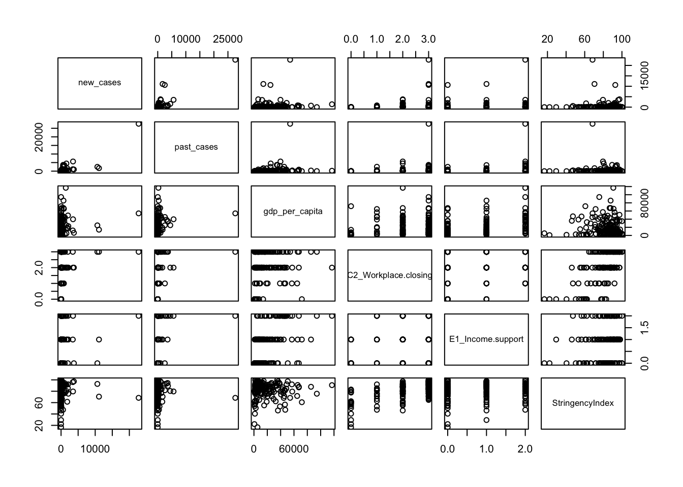
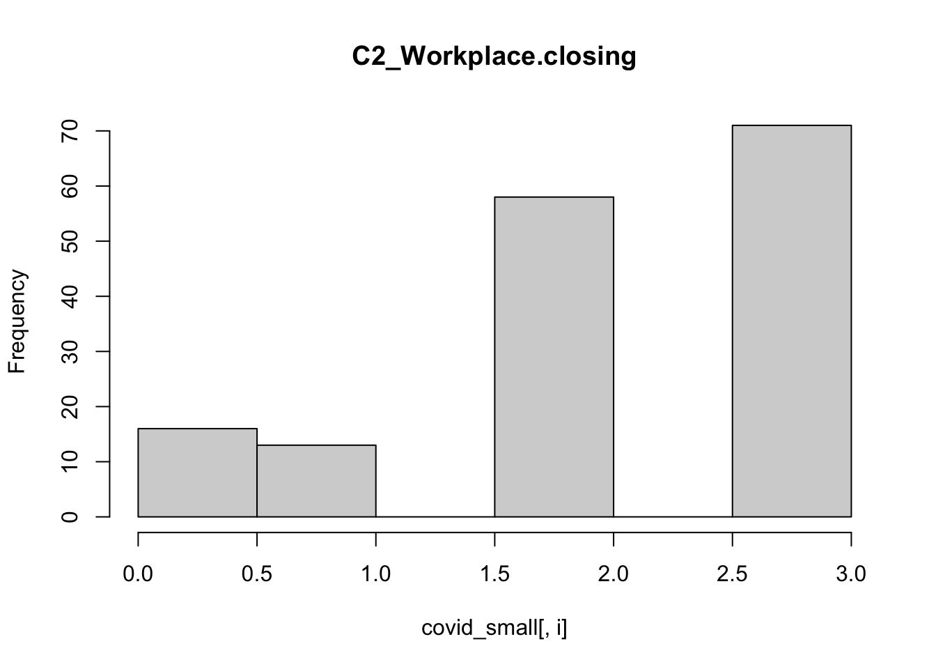
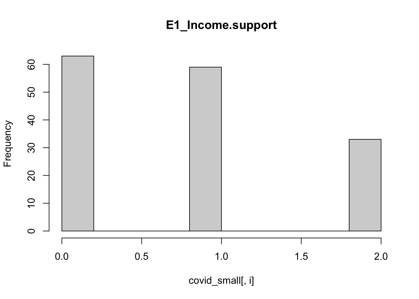
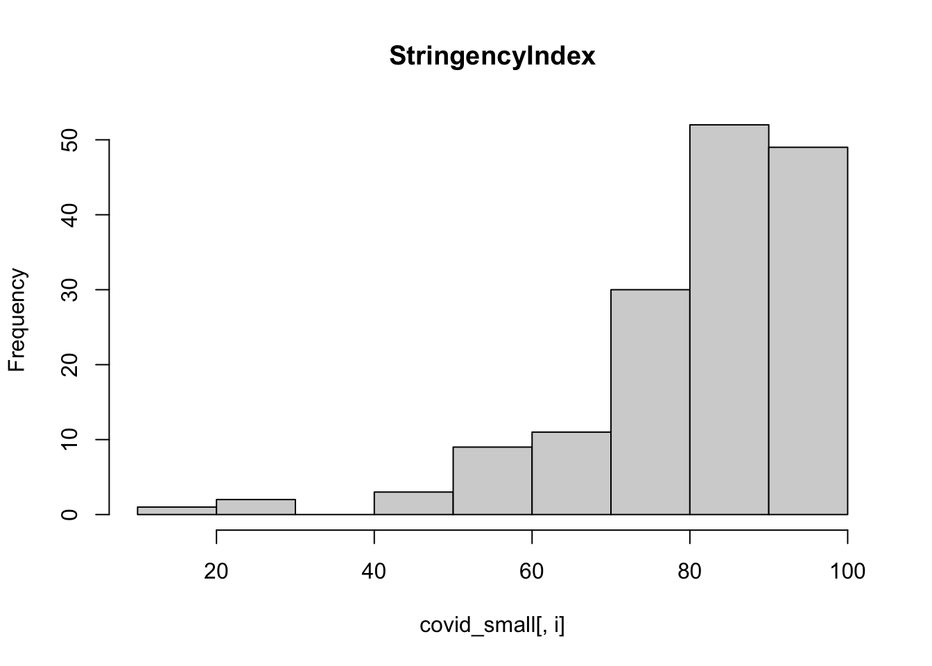
We can also use a for loop to plot a histogram for each column. The function ncol() retrieves the number of columns of a data.frame, and we will use it to loop from column 3 to the last one.
for (i in 3:ncol(covid_small)){
  hist(covid_small[,i],main = colnames(covid_small)[i])
}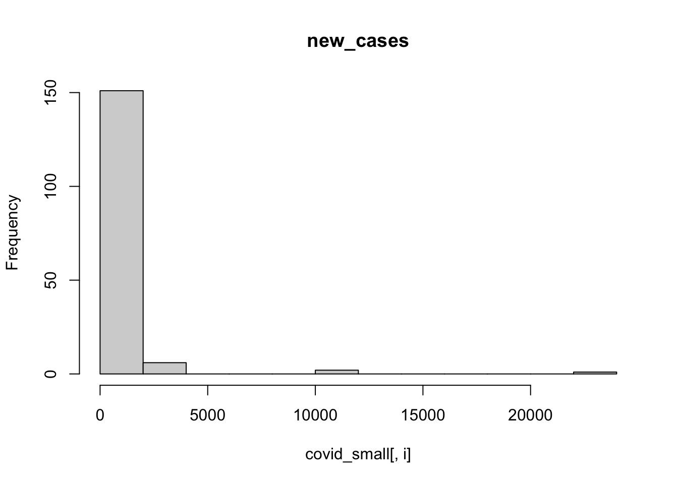
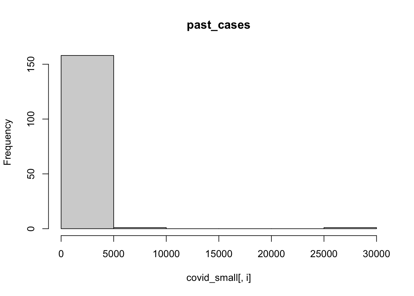
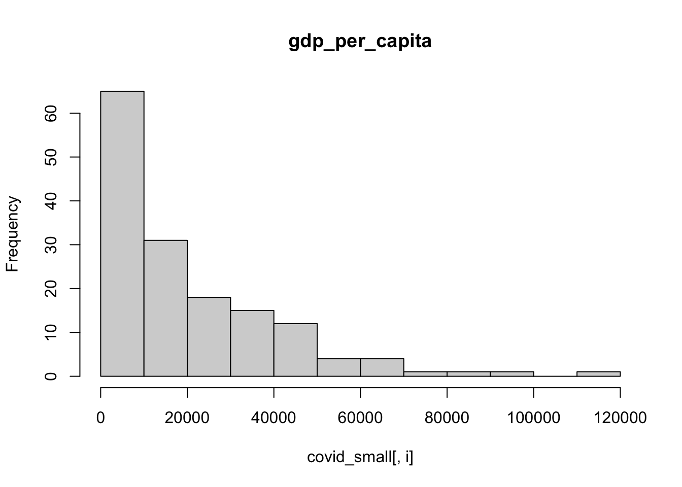
It is hard to visualize number of cases in the linear scale like this, let’s try doing a histogram of the logs:
hist(log10(covid_small[,3]), main = colnames(covid_small)[3])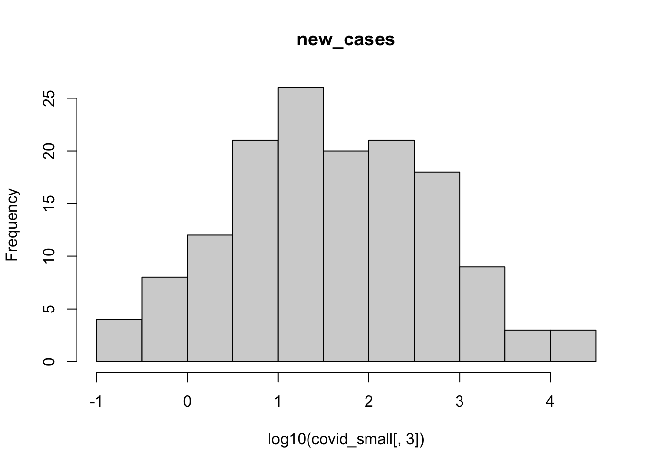
hist(log10(covid_small[,4]), main = colnames(covid_small)[4])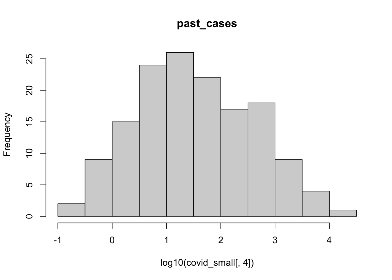
A few observations of this initial exploration:
- It will probably be a good idea to log-transform the number of cases, since they vary over orders of magnitude
- It also seems that the number of new cases is highly correlated with number of cases 2 weeks ago, so we always have to take that into account.
- Some of our possible independent variables seem to be correlated: richer countries seem to have closed schools more often, for example.
It is always good to visualize your dataset before starting to do inferences, so you will know how to best build your and models interpret them!
Before we proceed, let’s prepare the dataset we will use throughout the tutorial for linear models. We need to make sure all data columns have the appropriate type. For linear models, type matters, and specifically we have three important types:
numeric: columns with this type will be treated as a continuous variable. Example: number of cases.unordered factor: columns with this type will be treated as categorical variables. Example: world regionordered factor: columns with this type will be treated as ordinal variables. Example: Stringency of workplace closing
Let’s use str() to figure out the current data types for our columns and change as needed.
str(covid_small)## 'data.frame': 160 obs. of 8 variables:
## $ country_name : chr "Aruba" "Afghanistan" "Angola" "Albania" ...
## $ world_region : chr "Latin America and the Caribbean" "Asia and the Pacific" "Africa" "Europe" ...
## $ new_cases : num 0 400 0.6 9.6 1.2 ...
## $ past_cases : num 1.4 52.6 0 15.6 14.4 401 91.4 44 162 52.4 ...
## $ gdp_per_capita : num 35974 1804 5819 11803 NA ...
## $ C2_Workplace.closing: int 3 3 2 2 2 2 2 2 2 3 ...
## $ E1_Income.support : int 0 0 0 2 2 0 1 1 2 2 ...
## $ StringencyIndex : num 83.5 76.3 86.8 88.4 59.1 ...Country name and world region are currently characters. R will automatically convert them to unordered factors when we fit a model, but it is good practice to be explicit. Let’s change them to factors.
covid_small$country_name <- factor(covid_small$country_name)
covid_small$world_region <- factor(covid_small$world_region)
Stringency Index, gdp per capita and numbers of cases are currently numeric, as they should be, so we will do nothing.
International travel controls and Income support are currently considered as integer numbers, but they are not quite. They are ordinal variables encoded as numbers. Let’s transform them into ordered factors:
covid_small$E1_Income.support <- factor(covid_small$E1_Income.support, ordered = T)

covid_small$C2_Workplace.closing <- factor(covid_small$C2_Workplace.closing, ordered = T)
Let’s look at the data now:
str(covid_small)## 'data.frame': 160 obs. of 8 variables:
## $ country_name : Factor w/ 160 levels "Afghanistan",..: 7 1 5 2 4 150 6 8 9 10 ...
## $ world_region : Factor w/ 6 levels "Africa","Asia and the Pacific",..: 4 2 1 3 3 6 4 2 3 3 ...
## $ new_cases : num 0 400 0.6 9.6 1.2 ...
## $ past_cases : num 1.4 52.6 0 15.6 14.4 401 91.4 44 162 52.4 ...
## $ gdp_per_capita : num 35974 1804 5819 11803 NA ...
## $ C2_Workplace.closing: Ord.factor w/ 4 levels "0"<"1"<"2"<"3": 4 4 3 3 3 3 3 3 3 4 ...
## $ E1_Income.support : Ord.factor w/ 3 levels "0"<"1"<"2": 1 1 1 3 3 1 2 2 3 3 ...
## $ StringencyIndex : num 83.5 76.3 86.8 88.4 59.1 ...Seems better. Treating columns as factors also allow us to change the names of their levels to something more informative. Using the key above, let’s do it wiht income support. Currently, level names are 0, 1 and 2. Let’s change to none, less than 50% and more than 50%.
levels(covid_small$E1_Income.support) <- c('none',
                                          'less than 50%',
                                          'more than 50%')
Now let’s check:
str(covid_small)## 'data.frame': 160 obs. of 8 variables:
## $ country_name : Factor w/ 160 levels "Afghanistan",..: 7 1 5 2 4 150 6 8 9 10 ...
## $ world_region : Factor w/ 6 levels "Africa","Asia and the Pacific",..: 4 2 1 3 3 6 4 2 3 3 ...
## $ new_cases : num 0 400 0.6 9.6 1.2 ...
## $ past_cases : num 1.4 52.6 0 15.6 14.4 401 91.4 44 162 52.4 ...
## $ gdp_per_capita : num 35974 1804 5819 11803 NA ...
## $ C2_Workplace.closing: Ord.factor w/ 4 levels "0"<"1"<"2"<"3": 4 4 3 3 3 3 3 3 3 4 ...
## $ E1_Income.support : Ord.factor w/ 3 levels "none"<"less than 50%"<..: 1 1 1 3 3 1 2 2 3 3 ...
## $ StringencyIndex : num 83.5 76.3 86.8 88.4 59.1 ...Let’s do the same for International Travel controls:
levels(covid_small$C2_Workplace.closing) <- c('none',
                                             'recommend',
                                             'require some',
                                             'require most')
Finally, let’s change the names of some variables to something shorter and easier to type. Current names are:
colnames(covid_small)## [1] "country_name" "world_region" "new_cases"
## [4] "past_cases" "gdp_per_capita" "C2_Workplace.closing"
## [7] "E1_Income.support" "StringencyIndex"Let’s change some of them by using their index:
colnames(covid_small)[6] <- 'work_close'

colnames(covid_small)[7] <- 'income_support'

colnames(covid_small)[8] <- 'stringency_idx'
Now let’s look at our dataset:
str(covid_small)## 'data.frame': 160 obs. of 8 variables:
## $ country_name : Factor w/ 160 levels "Afghanistan",..: 7 1 5 2 4 150 6 8 9 10 ...
## $ world_region : Factor w/ 6 levels "Africa","Asia and the Pacific",..: 4 2 1 3 3 6 4 2 3 3 ...
## $ new_cases : num 0 400 0.6 9.6 1.2 ...
## $ past_cases : num 1.4 52.6 0 15.6 14.4 401 91.4 44 162 52.4 ...
## $ gdp_per_capita: num 35974 1804 5819 11803 NA ...
## $ work_close : Ord.factor w/ 4 levels "none"<"recommend"<..: 4 4 3 3 3 3 3 3 3 4 ...
## $ income_support: Ord.factor w/ 3 levels "none"<"less than 50%"<..: 1 1 1 3 3 1 2 2 3 3 ...
## $ stringency_idx: num 83.5 76.3 86.8 88.4 59.1 ...Looks good! The only step left is to remove NAs from the data. As we have seen in the second lesson, we can do it later when we will actually use the data, and this might be the best approach if there is a lot of scattered missing data. This is because na.omit on the whole data.frame will remove all rows with data missing for at least one column. In this dataset only 12 of the 160 countries included have missing datain some variable, so it won’t hurt much to remove these countries now so we do not need to think about it anymore.
covid_small <- na.omit(covid_small)The data is ready, let’s start modeling.
Fitting a model with categorical variables using formulas
The syntax that R uses to fit a model are formulas. We have seen formulas before, using them in plots in tutorial 3 and to fit models in tutorial 2. Let’s explain formulas a bit more here. You can get more help on formulas by using the help function:
help(formula)The basic syntax of a formula is:
response ~ predictorThis means that a variable named response depeends (~) on a variable named predictor. We can also use formulas with more than one variable as predictor, by using a plus sign:
response ~ predictor1 + predictor2This means that the variable response depends on predictor1 and predictor2, and that the effect of each predictor variable is independent of each other.
If the effect of predictors not only add to each other but also interact to generate the response, we can indicate that with an asterisk:
response ~ predictor1 * predictor2This means that the two predictors interact with each other and also have individual effects.
It is also possible to indicate in a formula that a variable is nested within another. Let’s imagine that you repeated an experiment in several locations and that you want to indicate that, a common formula would be:
response ~ predictor %in% locationFinally, you can include mathematical expressions in formulas. Let’s say you want to log-transform your response variable, for example. You can write this as:
log(response) ~ predictorThere are more things you can do with formulas, but let’s stop here for now and see it in practice. Let’s start by using a linear model to check whether the number of total cases varies between world regions. First, as we recommended before, let’s visualize whether this seems to be the case by using a boxplot. Both boxplots and linear models can take formulas!
boxplot(formula = new_cases ~ world_region, data = covid_small)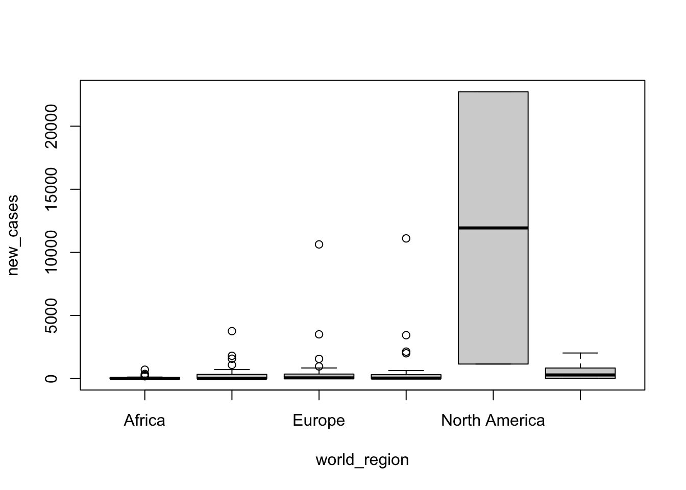
It seems it does, but it might be easier to visualize with a log scale. With base R, we use the parameter log='y' to indicate that we want a log scale on the y axis:
boxplot(formula = new_cases ~ world_region, data = covid_small, log='y')## Warning in plot.window(xlim = xlim, ylim = ylim, log = log, yaxs = pars$yaxs):
## nonfinite axis limits [GScale(-inf,4.3564,2, .); log=1]
Oops, there was an error! The reason is that some countries have 0 new cases in the past 5 days, and \(log(0)\) is undefined. In base R, there is no way to correct this with graph scales (we will see below how to do with ggplot). However, we can add the log transformation to the formula and pass to boxplot() the transformed data instead of the raw data. A typical log transformation when there are 0 values is \(log_{10}(x+1)\):
boxplot(formula = log10(new_cases+1) ~ world_region, data = covid_small)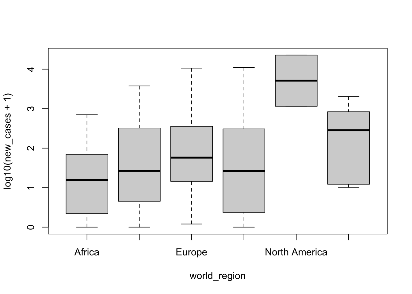
It seems there are variations between regions, but North America has many more cases. Is that difference significant? We will use a linear model to test. The syntax is similar that what we used to build the boxplot, but we will use the function lm():
region_model <- lm(formula = new_cases ~ world_region, data = covid_small)To check the results of our model fit, we can use the function summary:
summary(region_model)##
## Call:
## lm(formula = new_cases ~ world_region, data = covid_small)
##
## Residuals:
## Min 1Q Median 3Q Max
## -10784.4 -536.8 -311.7 -39.6 10784.4
##
## Coefficients:
## Estimate Std. Error t value
## (Intercept) 62.97 290.34 0.217
## world_regionAsia and the Pacific 327.72 464.14 0.706
## world_regionEurope 501.52 418.42 1.199
## world_regionLatin America and the Caribbean 689.28 459.06 1.501
## world_regionNorth America 11872.23 1361.80 8.718
## world_regionWest Asia 502.81 662.07 0.759
## Pr(>|t|)
## (Intercept) 0.829
## world_regionAsia and the Pacific 0.481
## world_regionEurope 0.233
## world_regionLatin America and the Caribbean 0.135
## world_regionNorth America 6.76e-15 ***
## world_regionWest Asia 0.449
## ---
## Signif. codes: 0 '***' 0.001 '**' 0.01 '*' 0.05 '.' 0.1 ' ' 1
##
## Residual standard error: 1882 on 142 degrees of freedom
## Multiple R-squared: 0.3502, Adjusted R-squared: 0.3273
## F-statistic: 15.3 on 5 and 142 DF, p-value: 5.082e-12Summary shows a few different things about the model. For now, let’s pay attention to the coefficients table. This is a table with the estimates for all components of our model, and the p-value of each coefficient. When the predictor is an unordered factor, it uses the first level of the factor as the intercept. Here it is Africa, which is considered our baseline, and the other estimated coefficients denote the difference between each region and Africa. It seems that North America is significantly different from Africa, while the other regions are not.
However, before we jump to conclusions, we have to answer two questions first to check if our interpretation is valid: 1. does this model fit our assumptions about the data? 2. do we need world regions at all to explain differences between countries?
To answer the first question, we need to evaluate our model fit, and R has several tools for that
Evaluate model fit
Let’s call the summary function again to talk about another part of the output:
summary(region_model)##
## Call:
## lm(formula = new_cases ~ world_region, data = covid_small)
##
## Residuals:
## Min 1Q Median 3Q Max
## -10784.4 -536.8 -311.7 -39.6 10784.4
##
## Coefficients:
## Estimate Std. Error t value
## (Intercept) 62.97 290.34 0.217
## world_regionAsia and the Pacific 327.72 464.14 0.706
## world_regionEurope 501.52 418.42 1.199
## world_regionLatin America and the Caribbean 689.28 459.06 1.501
## world_regionNorth America 11872.23 1361.80 8.718
## world_regionWest Asia 502.81 662.07 0.759
## Pr(>|t|)
## (Intercept) 0.829
## world_regionAsia and the Pacific 0.481
## world_regionEurope 0.233
## world_regionLatin America and the Caribbean 0.135
## world_regionNorth America 6.76e-15 ***
## world_regionWest Asia 0.449
## ---
## Signif. codes: 0 '***' 0.001 '**' 0.01 '*' 0.05 '.' 0.1 ' ' 1
##
## Residual standard error: 1882 on 142 degrees of freedom
## Multiple R-squared: 0.3502, Adjusted R-squared: 0.3273
## F-statistic: 15.3 on 5 and 142 DF, p-value: 5.082e-12Another information given by summary() is the distribution of residuals. Residuals are the variation that cannot be explained by the model: the difference between what our model predicts and what we actually observe. For example, in the coefficients table we see that the coefficient estimated for Africa (the model intercept) is 62.97. So the model estimates that an African country would have an average of 62.97 new cases of covid19 now. Let’s look at how many cases they actually have by plotting each country as a point.
We will use ggplot this time since it is more flexible. For example, instead of transforming the data we can tell it to use a transformation of log plus one for the y axis. We will also plot a straight line at the intercept, which is the inference for Africa, so we can compare the distribution of points.
Let’s first load the package.
library(ggplot2)And now we can plot.
Africa_only <- covid_small[covid_small$world_region =='Africa', ]

ggplot(Africa_only) +
  geom_point(aes(x = world_region, y = new_cases)) +
  scale_y_continuous(trans='log1p', breaks = c(1,10,100)) +
  geom_hline(yintercept = 62.97, color = 'red')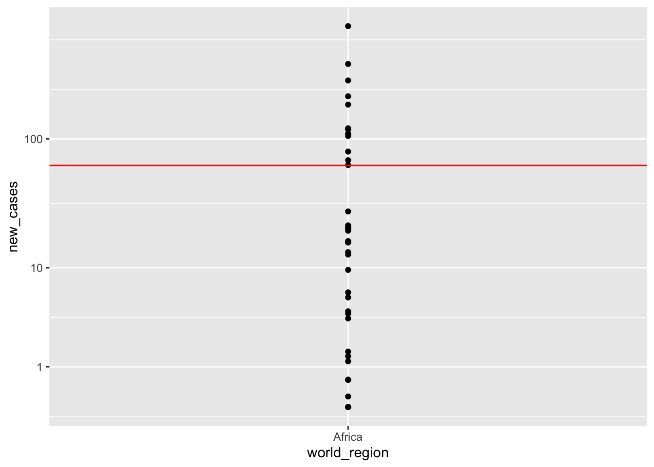
Here we can see two things:
- We slightly overstimated the number of cases for Africa
- There is a large variation within Africa. The differences between an actual African country and our estimate are the residuals.
In a typical linear model, we assume that the residuals should be normally distributed, and that they follow the same distribution across all the data. In out case, it means that the residuals should be more or less the same for all world regions. Is that the case? R has a simple function to calculate residuals, named resid():
residuals <- resid(region_model)We saved the result of resid(region_model) in the object residuals, which is a vector with residual values:
str(residuals)## Named num [1:148] -752.25 9.31 -62.37 -554.89 160.82 ...
## - attr(*, "names")= chr [1:148] "1" "2" "3" "4" ...The result of this function is a vector that shows the residuals for each one of our data points. Let’s build a data.frame with our data and residuals to visualize if our assumptions about residuals hold:
resid_df <- data.frame(world_region = covid_small$world_region, residual = residuals)Let’s look at histograms of our residuals for each world region now:
ggplot(resid_df)+
  geom_histogram(aes(x=residuals)) +
  facet_wrap(~world_region,ncol = 2)
## `stat_bin()` using `bins = 30`. Pick better value with `binwidth`.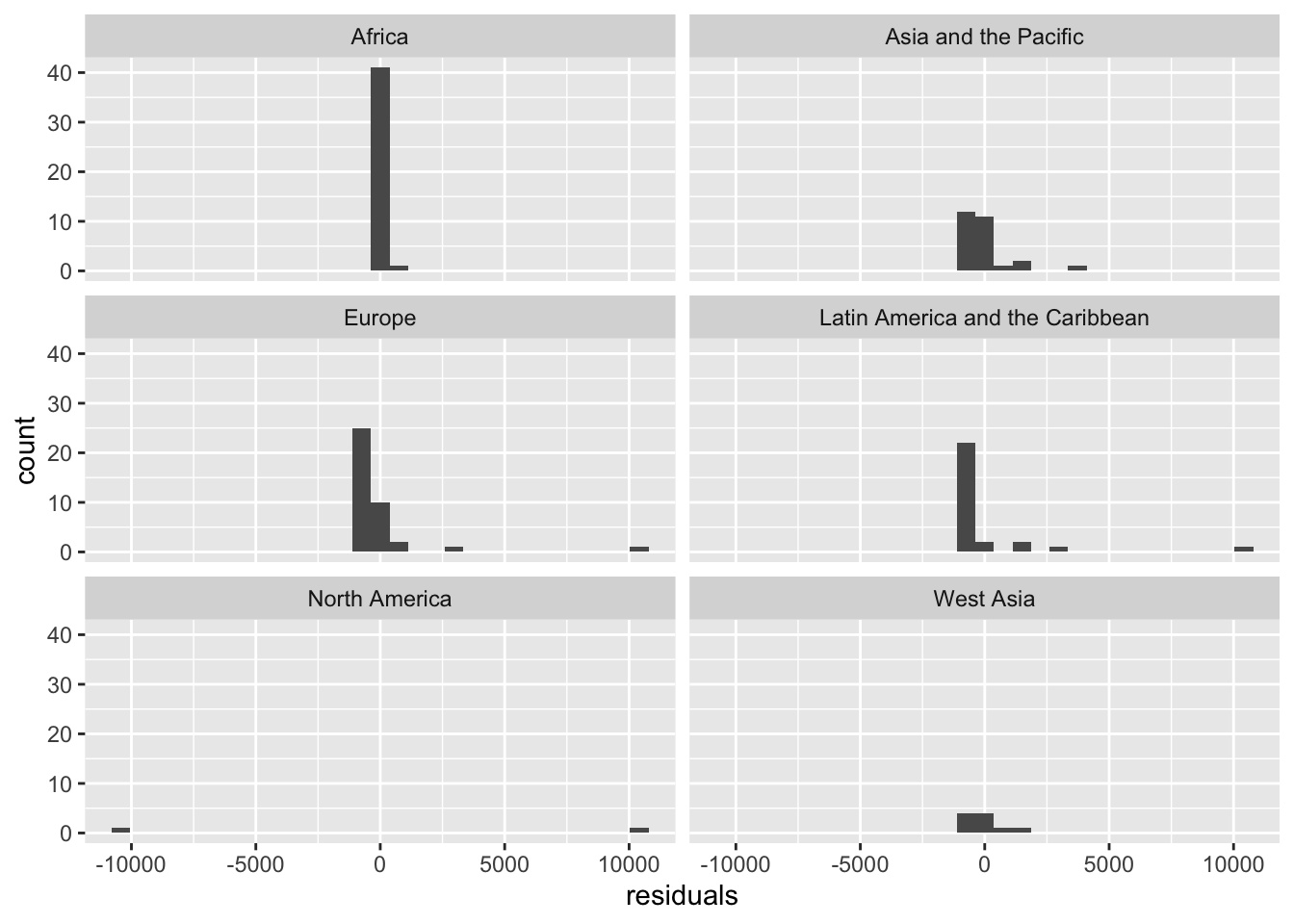
The residuals do not look normally distribued, and also not the same for all regions!
We did all this to get an intuition about how we evaluate model fit, but R has nice function to help us understand whether the model assumption holds. If we give our model as input to the function plot(), it will return a series of graphs:
plot(region_model)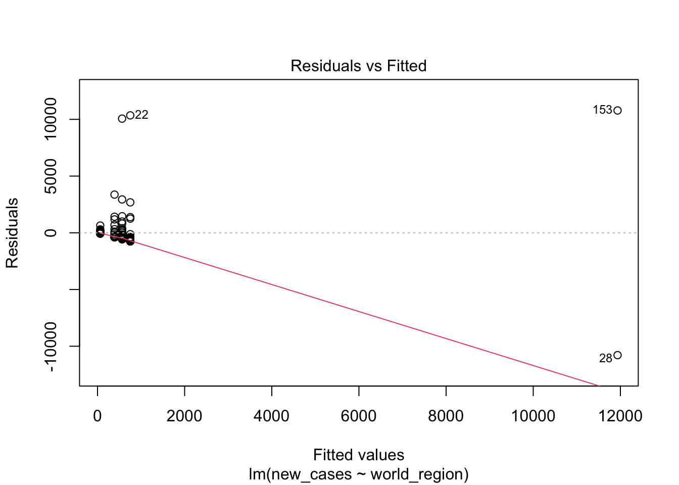
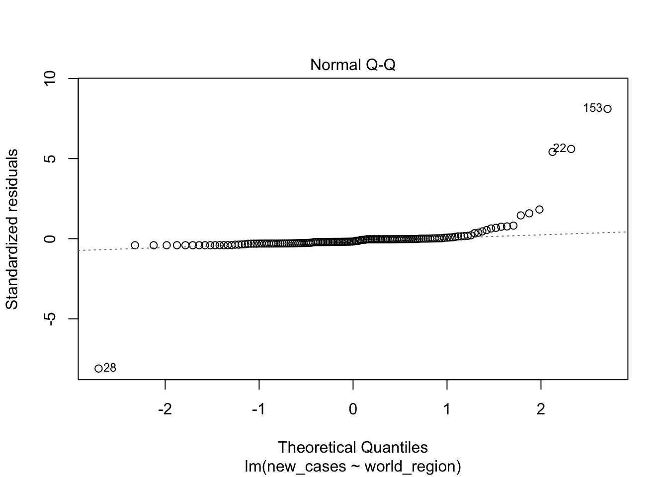
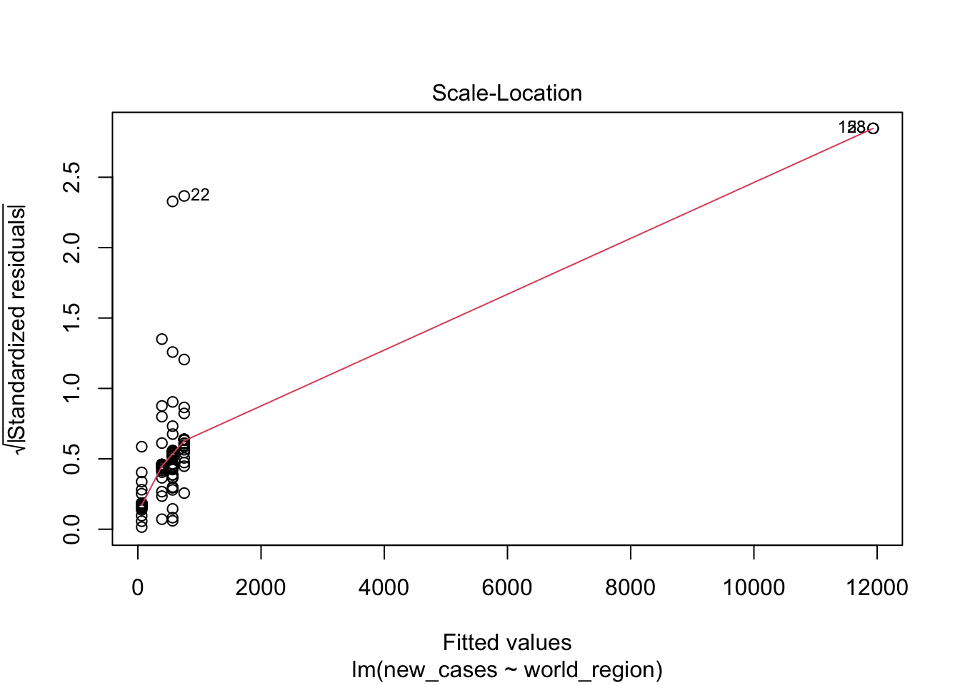
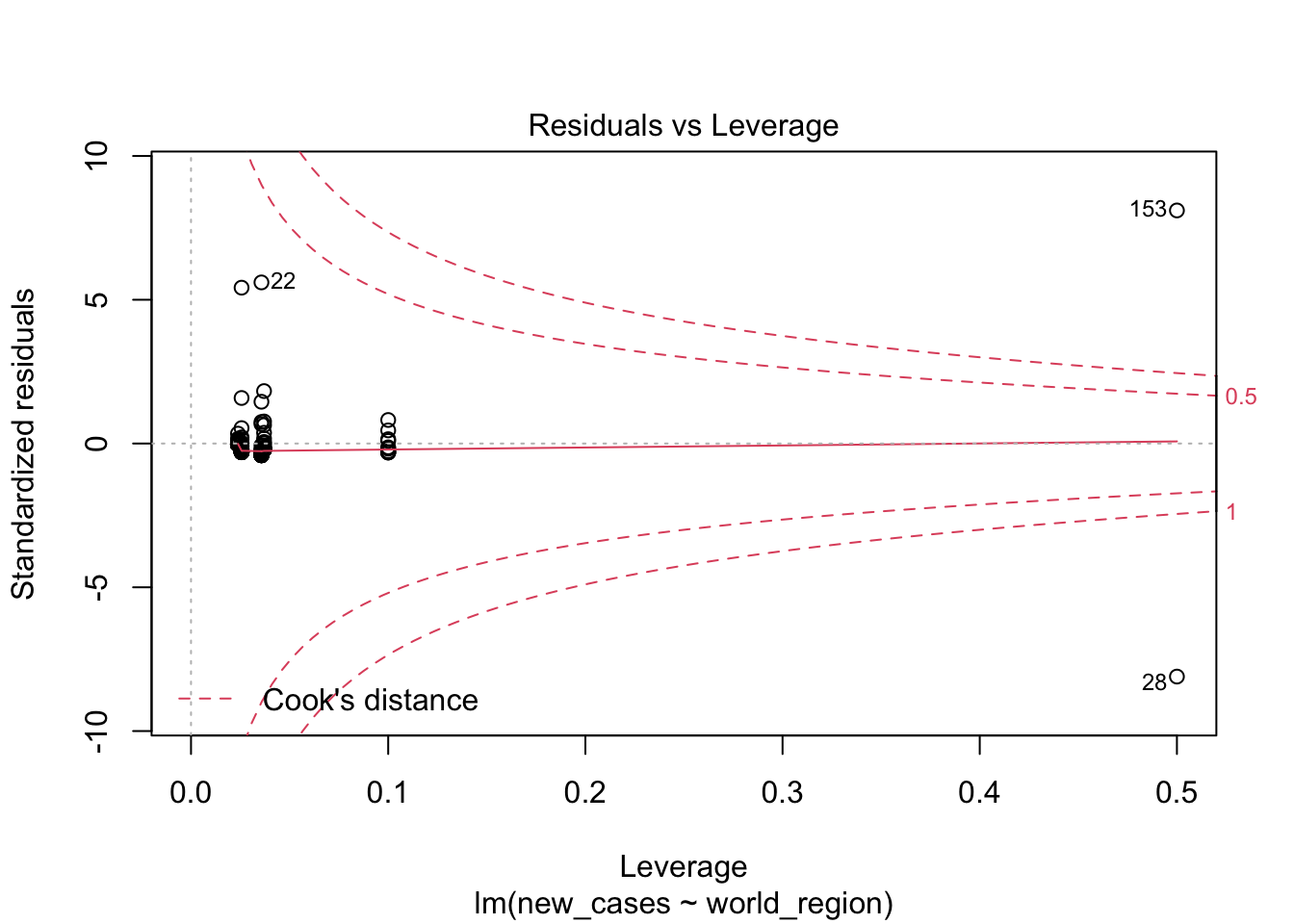
The first graph shows our fitted values (i. e., model predictions) against residuals. It seems the dispersion of residuals is increasing with increased fitted values. The average trend (red line) is decreasing. In a good model, there should be no trend and the variance should be constant.
The second graph is a Q-Q plot and compares our residuals to what would be expected if they were normally distributed. For a good model, it should be a straight line with slope of 1. This is far from what we are observing
The third graph is similar to the first one, but the y axis is the square root of residuals, with sign removed. Again, it indicates that the variation in residuals is increasing with higher predicted response
the fourth graphs helps to identify outliers, which are the labelled points farthest from the dashed region, and happen to be data points 22, 28 and 153. Which countries are these? These labels are the row names, not row numbers, so we need to provide a character vector to index them:
covid_small$country_name[c('22','28','153')]## [1] <NA> <NA> <NA>
## 160 Levels: Afghanistan Albania Algeria Andorra Angola Argentina ... ZimbabweThis is saying that these three data points are the ones that are most influencing the model. we might consider removing them if we can’t build a good model at all.
But before doing that, it seems we can improve our model by log-transforming the response variable. When variation in residuals increases with fitted values, this can often help.
Let’s try this.
region_model_log <- lm(formula = log(new_cases) ~ world_region, data = covid_small)## Error in lm.fit(x, y, offset = offset, singular.ok = singular.ok, ...): NA/NaN/Inf in 'y'Oops, we got an error. This is because some countries have a number of cases of 0, so we cannot calculate the log. As we did with the graph, we can do a slightly different transformation and add 1 to all countries:
region_model_log <- lm(formula = log(new_cases+1) ~ world_region, data = covid_small)Now let’s plot the model to check the model fit:
plot(region_model_log)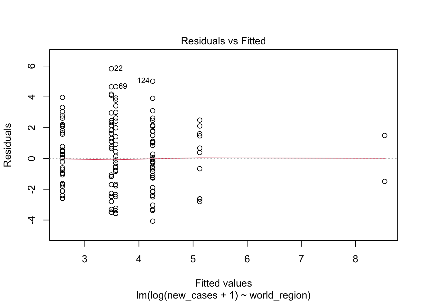
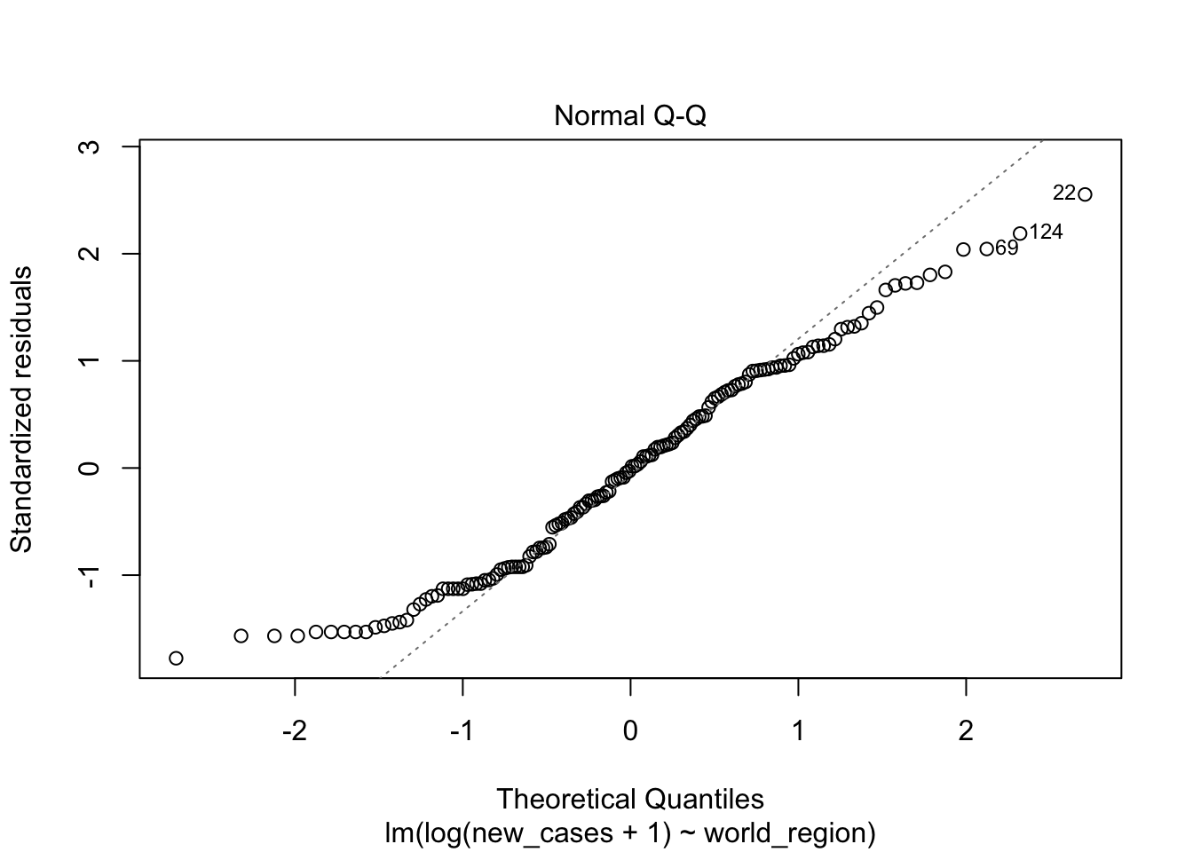
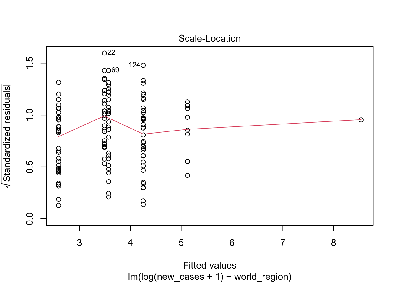
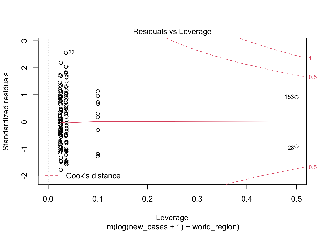
It seems much better! The variation in residuals seems more or less constant across fitted values, the q-q plot is closer to a straight line and there are no points outside the dashed region in the last plot.
Has this log transformation changed anything about our estimates? Let’s use summary to figure out:
summary(region_model_log)##
## Call:
## lm(formula = log(new_cases + 1) ~ world_region, data = covid_small)
##
## Residuals:
## Min 1Q Median 3Q Max
## -4.0715 -2.1173 -0.0149 1.7933 5.8240
##
## Coefficients:
## Estimate Std. Error t value
## (Intercept) 2.5873 0.3584 7.219
## world_regionAsia and the Pacific 0.9848 0.5730 1.719
## world_regionEurope 1.6666 0.5165 3.226
## world_regionLatin America and the Caribbean 0.9039 0.5667 1.595
## world_regionNorth America 5.9528 1.6811 3.541
## world_regionWest Asia 2.5359 0.8173 3.103
## Pr(>|t|)
## (Intercept) 2.91e-11 ***
## world_regionAsia and the Pacific 0.08784 .
## world_regionEurope 0.00156 **
## world_regionLatin America and the Caribbean 0.11295
## world_regionNorth America 0.00054 ***
## world_regionWest Asia 0.00231 **
## ---
## Signif. codes: 0 '***' 0.001 '**' 0.01 '*' 0.05 '.' 0.1 ' ' 1
##
## Residual standard error: 2.323 on 142 degrees of freedom
## Multiple R-squared: 0.147, Adjusted R-squared: 0.1169
## F-statistic: 4.892 on 5 and 142 DF, p-value: 0.000368Now we gained much more power to find the differences. It seems most regions are different from Africa, with Latin America and Caribbean being more similar. Also notice that the estimates are different, because now we are modeling the log-transformed covid19 cases. This is not important now, but will be for prediction, which we will see below.
Before proceeding, let’s note that the choice of intercept for categorical variables is arbitrary. R chooses one arbitrary level in a factor as the intercept. To choose the baseline comparison yourself, you can explicitly set the reference level. Let’s set Latin America and the Caribbean using the function relevel():
covid_small$world_region <- relevel(covid_small$world_region,
                                    ref = 'Latin America and the Caribbean' )
Now let’s fit a new model and print the summary. Latin America will be the intercept and all comparisons will be done in relation to it. Remember: this makes no difference for model predictions or for model test (which we will see below), just for which contrasts are displayed here!
region_model_log <- lm(formula = log(new_cases+1) ~ world_region, data = covid_small)

summary(region_model_log)
##
## Call:
## lm(formula = log(new_cases + 1) ~ world_region, data = covid_small)
##
## Residuals:
## Min 1Q Median 3Q Max
## -4.0715 -2.1173 -0.0149 1.7933 5.8240
##
## Coefficients:
## Estimate Std. Error t value Pr(>|t|)
## (Intercept) 3.49119 0.43898 7.953 5.18e-13 ***
## world_regionAfrica -0.90389 0.56671 -1.595 0.1129
## world_regionAsia and the Pacific 0.08093 0.62653 0.129 0.8974
## world_regionEurope 0.76267 0.57537 1.326 0.1871
## world_regionNorth America 5.04887 1.70014 2.970 0.0035 **
## world_regionWest Asia 1.63200 0.85572 1.907 0.0585 .
## ---
## Signif. codes: 0 '***' 0.001 '**' 0.01 '*' 0.05 '.' 0.1 ' ' 1
##
## Residual standard error: 2.323 on 142 degrees of freedom
## Multiple R-squared: 0.147, Adjusted R-squared: 0.1169
## F-statistic: 4.892 on 5 and 142 DF, p-value: 0.000368While summary() is a good function to display model results in R, it does not produce results that we can save as a csv and open, for example, in Excel to make a nice table for a paper. The R package broom contains functions to do that. Let’s load this package and use the function tidy to see the results. Remeber to install the package broom with install.packages('broom') if you do not have it already.
library(broom)
tidy(region_model_log)
## # A tibble: 6 x 5
## term estimate std.error statistic p.value
## <chr> <dbl> <dbl> <dbl> <dbl>
## 1 (Intercept) 3.49 0.439 7.95 5.18e-13
## 2 world_regionAfrica -0.904 0.567 -1.59 1.13e- 1
## 3 world_regionAsia and the Pacific 0.0809 0.627 0.129 8.97e- 1
## 4 world_regionEurope 0.763 0.575 1.33 1.87e- 1
## 5 world_regionNorth America 5.05 1.70 2.97 3.50e- 3
## 6 world_regionWest Asia 1.63 0.856 1.91 5.85e- 2Much better for saving! Let’s now assign this table to a variable and save it so we can open in Excel later.
nice_table <- tidy(region_model_log)
write.csv(nice_table, file = 'nice_table.csv')
Model choice
Now that we used a transformation and made sure that the model fits the normality assumption, we have one more step: to show that we need to consider region at all. It could be the case that differences between some regions exist only by chance, and that a single normal distribution without considering world region could adequately explain our data. To test whether this is the case, we will use the function drop1(), which will try to remove predictors from our model and test if the result is a better model:
drop1(region_model_log)## Single term deletions
##
## Model:
## log(new_cases + 1) ~ world_region
## Df Sum of Sq RSS AIC
## <none> 766.17 255.34
## world_region 5 131.99 898.16 268.86The function drop1 tries to remove each predictor from the model (in our case, it was just one!) and then calculates the Akaike Information Criteria (AIC), which is a statistic that tries to balance model complexity with explanatory power. The lower the value of AIC, the better a model is. Differences of AIC of 2 or more are typically considered very strong. What the table is saying here is that not removing any predictor (world_region.
Another way to test whether a predictor is important is by doing an F test, using the function anova():
anova(region_model_log)## Analysis of Variance Table
##
## Response: log(new_cases + 1)
## Df Sum Sq Mean Sq F value Pr(>F)
## world_region 5 131.99 26.3971 4.8923 0.000368 ***
## Residuals 142 766.17 5.3956
## ---
## Signif. codes: 0 '***' 0.001 '**' 0.01 '*' 0.05 '.' 0.1 ' ' 1Here the F-test resulted in a very small p-value for world_region, indicating that this term significantly improves the model.
Usually both methods will have similar results, but they might differ when the p-value is close to 0.05.
We can also do the F-test and calculate AICs at the same time by providing an additional argument to drop1():
drop1(region_model_log, test = 'F')## Single term deletions
##
## Model:
## log(new_cases + 1) ~ world_region
## Df Sum of Sq RSS AIC F value Pr(>F)
## <none> 766.17 255.34
## world_region 5 131.99 898.16 268.86 4.8923 0.000368 ***
## ---
## Signif. codes: 0 '***' 0.001 '**' 0.01 '*' 0.05 '.' 0.1 ' ' 1Ordered categorical variables and continuous variables
We saw above an example using a categorical variable as predictor, but we can also use ordered factors. For example, workplace closing:
str(covid_small$work_close)## Ord.factor w/ 4 levels "none"<"recommend"<..: 4 4 3 3 3 3 3 3 4 1 ...Let’s plot the relationship between both, log-transforming the number of cases:
plot(formula = log10(new_cases+1) ~ work_close, data = covid_small)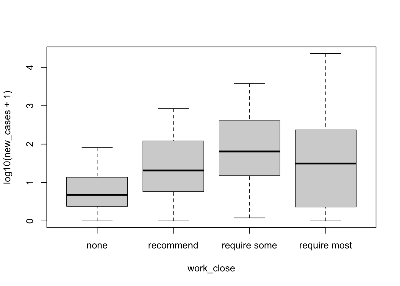
Maybe it has an effect, but not clear. It seems that this is a non-linear relationship that increases up until some point and then decreases.
model_work <- lm(formula = new_cases ~ work_close, data = covid_small)Let’s evaluate the model fit:
plot(model_work)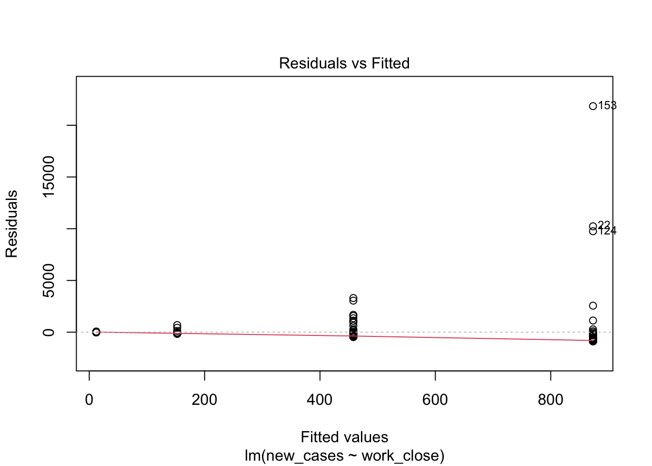
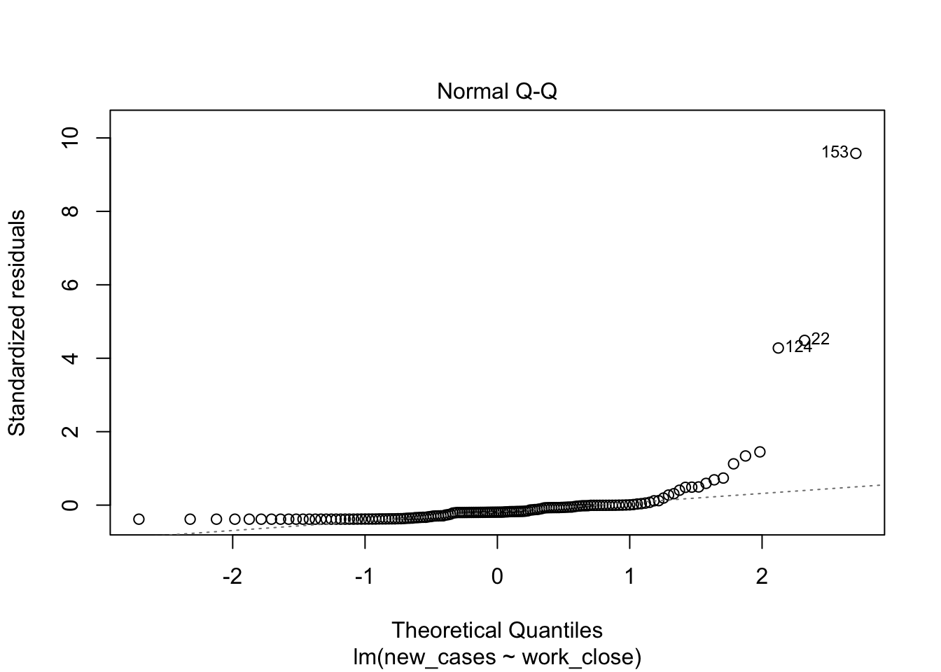
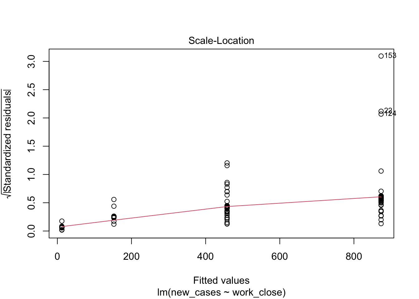
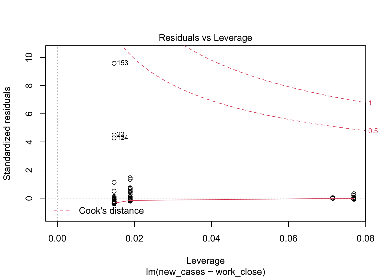
Model fit does not look good, let’s see if we can improve it with a log-transformation of the response variable:
model_work_log <- lm(formula = log(new_cases+1) ~ work_close, data = covid_small)

plot(model_work_log)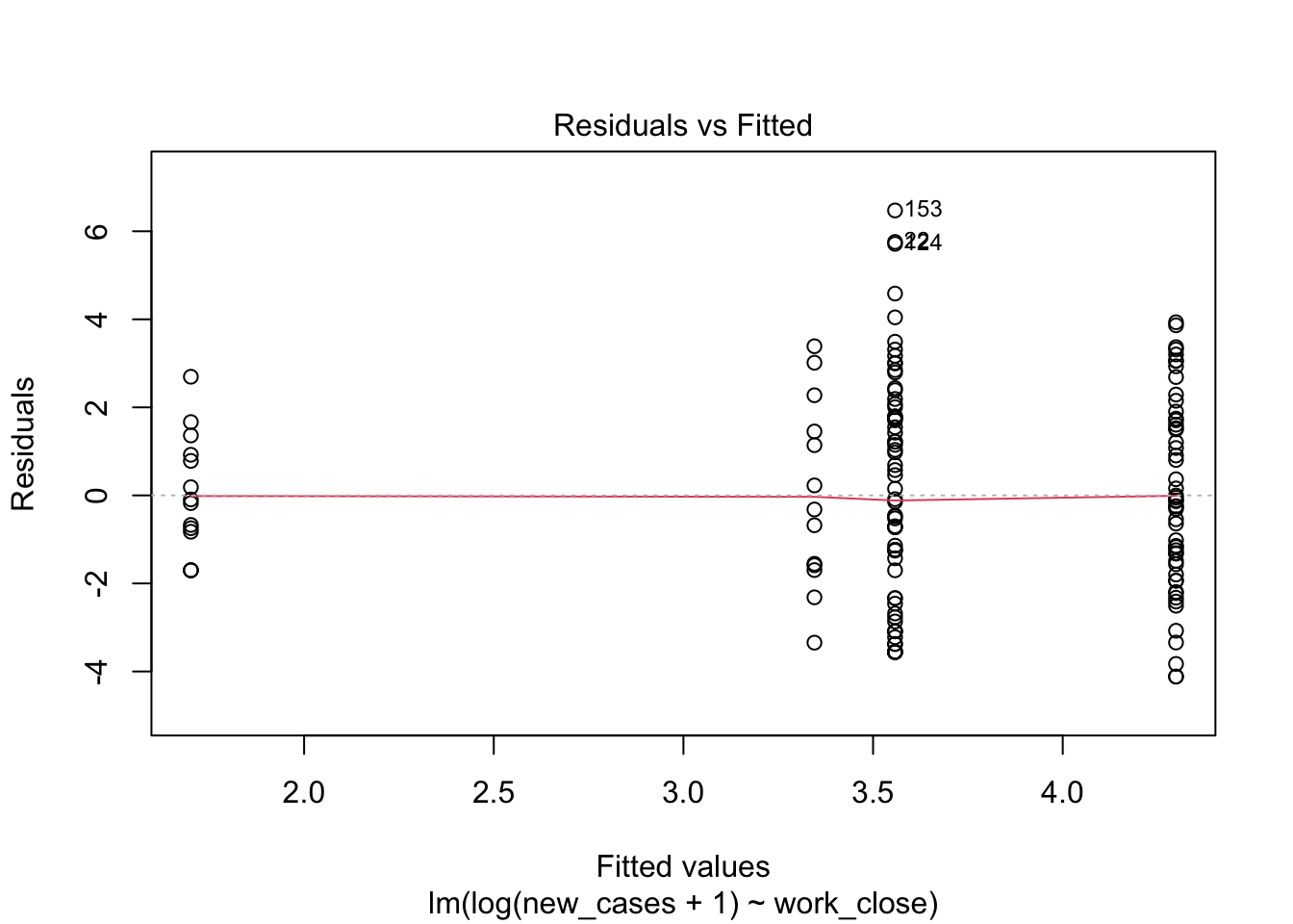
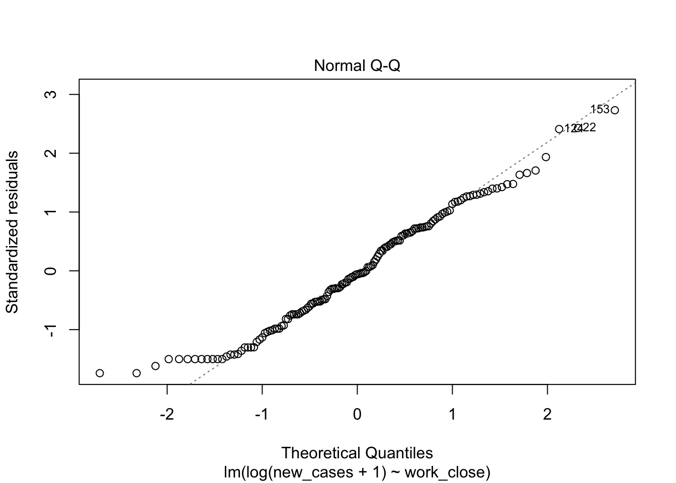
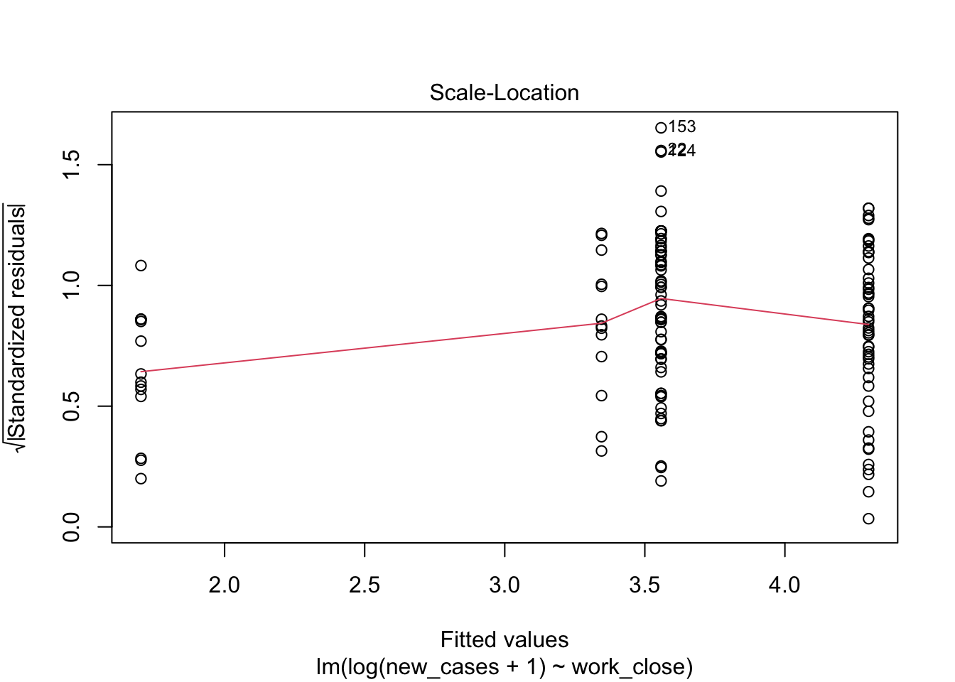
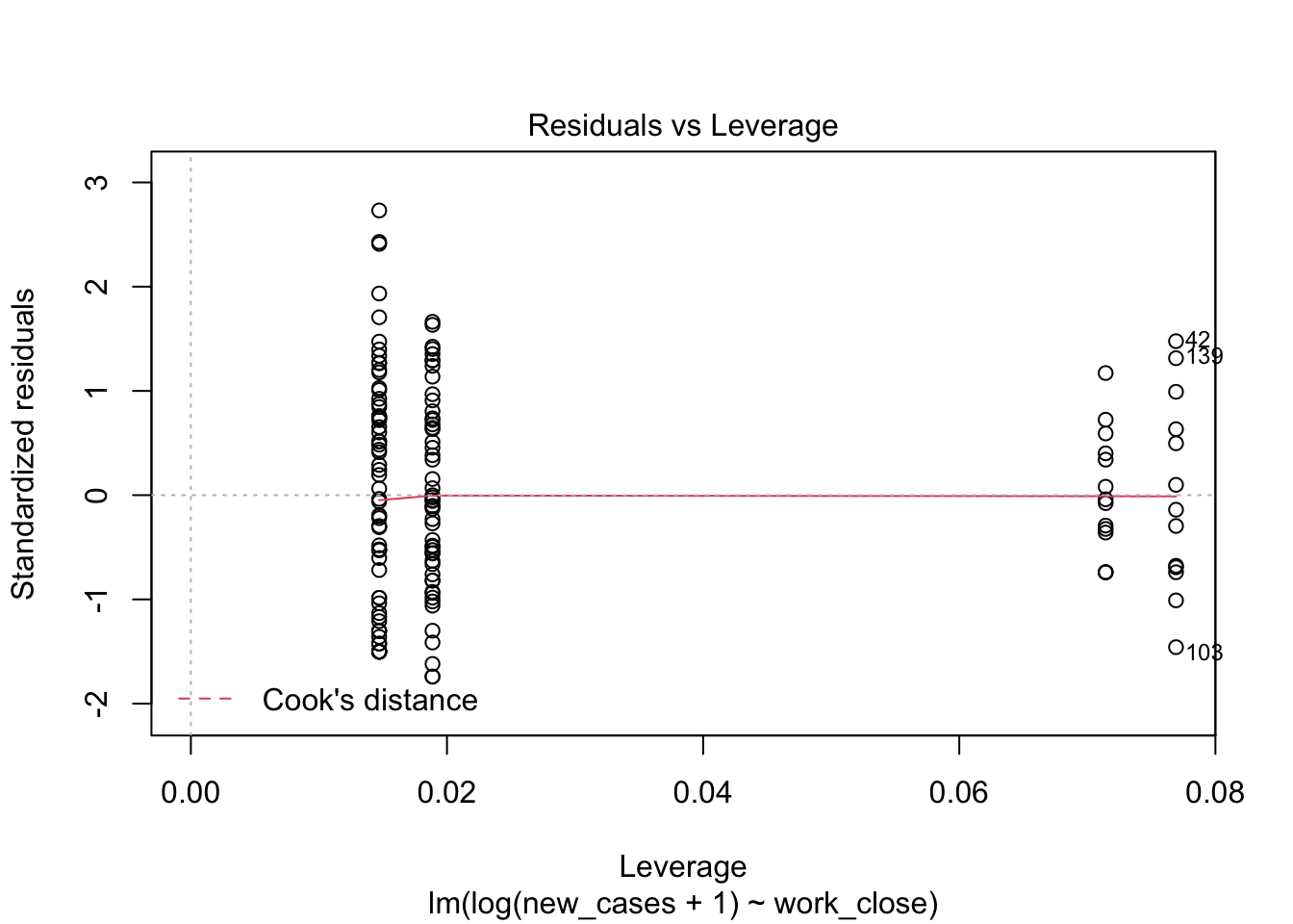
Much better. Let’s look at the summary now:
summary(model_work_log)##
## Call:
## lm(formula = log(new_cases + 1) ~ work_close, data = covid_small)
##
## Residuals:
## Min 1Q Median 3Q Max
## -4.1163 -1.7015 -0.1385 1.7441 6.4731
##
## Coefficients:
## Estimate Std. Error t value Pr(>|t|)
## (Intercept) 3.2259 0.2546 12.670 < 2e-16 ***
## work_close.L 1.4585 0.4983 2.927 0.00398 **
## work_close.Q -1.1923 0.5092 -2.342 0.02058 *
## work_close.C -0.2243 0.5199 -0.431 0.66677
## ---
## Signif. codes: 0 '***' 0.001 '**' 0.01 '*' 0.05 '.' 0.1 ' ' 1
##
## Residual standard error: 2.388 on 144 degrees of freedom
## Multiple R-squared: 0.08592, Adjusted R-squared: 0.06688
## F-statistic: 4.512 on 3 and 144 DF, p-value: 0.004677In the case of ordered factors, it is a little less intuitive to understand how R fits them, but basically they are treated as a number. Instead of fitting one parameter per factor level, it fits what we call a polynomial regression. work_close.L is the linear effect of travel control, indicating that the higher the stringency of workplace close orders, the lower the number of new cases. work_close.Q is the quadratic effect, which is negative, indicating a peak.work_close.C is the cubic effect, allowing the relationship between work_close and our response variable to be nonlinear.
Each estimated parameters is not as important for us now as whether travel control is important overall. For that, we use the function drop1().
drop1(model_work_log, test = 'F')## Single term deletions
##
## Model:
## log(new_cases + 1) ~ work_close
## Df Sum of Sq RSS AIC F value Pr(>F)
## <none> 820.99 261.57
## work_close 3 77.172 898.16 268.86 4.512 0.004677 **
## ---
## Signif. codes: 0 '***' 0.001 '**' 0.01 '*' 0.05 '.' 0.1 ' ' 1In this case, it seems that a model including workplace closings is much better than one that does not, and that closing workplaces generally increases the number of new coronavirus cases.
That seems counter-intuitive: does closing work places make the pandemics worse??? We will have a closer look in the next section.
Multiple predictors
The last example will be useful for us to introduce fitting models with multiple predictors. We can imagine, for example, that the effect that we found could be spurious, and workplace restrictions are actually associated with another variable that is the true driver of new covid19 cases. For example, it could be that countries decided to close workplaces based on how severe covid19 was a month ago, and that the number of past cases is really the main factor explaining current trends.
We can fit a new regression including past cases as a predictor and test if, considering past cases, workplace closings are still important.
We can use ggplot to visualize the effect of both variables at the same time. The number of past cases will be the X axis, while work closures will be color-coded:
ggplot(covid_small) +
  geom_point(aes(x = past_cases, y = new_cases, color = work_close)) +
  scale_x_continuous(trans = 'log1p', breaks = 10^(0:5)) +
scale_y_continuous(trans = 'log1p', breaks = 10^(0:5)) 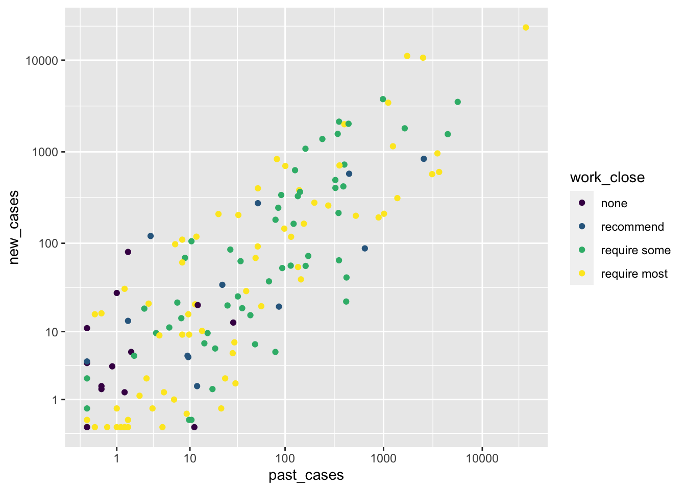
With this plot, it now becomes clear that the number of new cases is determined by the number of past cases. It does not look like work closures have much influence other than that. More importantly, we should be cautious: all countries with more than 100 cases seem to have adopted some sort of workplace closure intervention, most of them with the more strict controls. That means that we will have little power to actually detect any effect of work closures! If this were an experiment, we should have better balanced the different treatments. Since this is not an experiment but rather observations, we will move on, knowing that this imbalance will impact our ability to detect differences.
Now we can fit the model, evaluate it and test with drop1():
model_work_past <- lm(formula = log(new_cases+1) ~ log(past_cases+1) + work_close,
                      data = covid_small)
plot(model_work_past)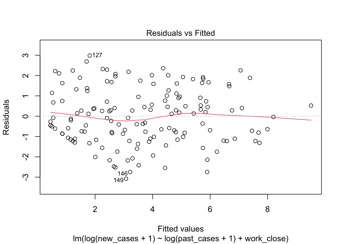
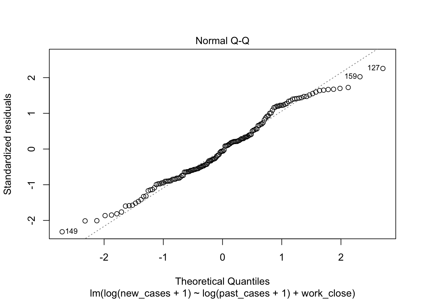

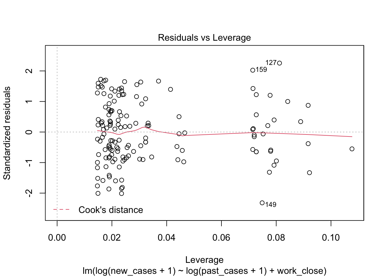
drop1(model_work_past, test = 'F')## Single term deletions
##
## Model:
## log(new_cases + 1) ~ log(past_cases + 1) + work_close
## Df Sum of Sq RSS AIC F value Pr(>F)
## <none> 272.19 100.176
## log(past_cases + 1) 1 548.79 820.99 261.567 288.3172 <2e-16 ***
## work_close 3 1.84 274.03 95.173 0.3224 0.8092
## ---
## Signif. codes: 0 '***' 0.001 '**' 0.01 '*' 0.05 '.' 0.1 ' ' 1In this case, the lowest AIC is a model without work closures (notice that the table is NOT ordered by AIC). The F test also did not find a significant difference between a model deleting no variable and a model deleting work_close. Since they are not statistically different, we use the parsimony principle and keep the simpler model.
Now we will fit a new model, withut work_close, and do the test again to see if deleting past_cases improves the model further.
model_pastonly <- lm(formula = log(new_cases+1) ~ log(past_cases+1), data = covid_small)drop1(model_pastonly, test = 'F')## Single term deletions
##
## Model:
## log(new_cases + 1) ~ log(past_cases + 1)
## Df Sum of Sq RSS AIC F value Pr(>F)
## <none> 274.03 95.173
## log(past_cases + 1) 1 624.13 898.16 268.864 332.52 < 2.2e-16 ***
## ---
## Signif. codes: 0 '***' 0.001 '**' 0.01 '*' 0.05 '.' 0.1 ' ' 1Now the difference is significant: we cannot improve our model by removing any more terms.
We can now use summary(), tidy(), plot() and all functions shown above to the result of step():
summary(model_pastonly)##
## Call:
## lm(formula = log(new_cases + 1) ~ log(past_cases + 1), data = covid_small)
##
## Residuals:
## Min 1Q Median 3Q Max
## -2.83253 -0.97520 0.06853 1.03690 2.98861
##
## Coefficients:
## Estimate Std. Error t value Pr(>|t|)
## (Intercept) 0.57470 0.20183 2.847 0.00504 **
## log(past_cases + 1) 0.87242 0.04784 18.235 < 2e-16 ***
## ---
## Signif. codes: 0 '***' 0.001 '**' 0.01 '*' 0.05 '.' 0.1 ' ' 1
##
## Residual standard error: 1.37 on 146 degrees of freedom
## Multiple R-squared: 0.6949, Adjusted R-squared: 0.6928
## F-statistic: 332.5 on 1 and 146 DF, p-value: < 2.2e-16plot(model_pastonly)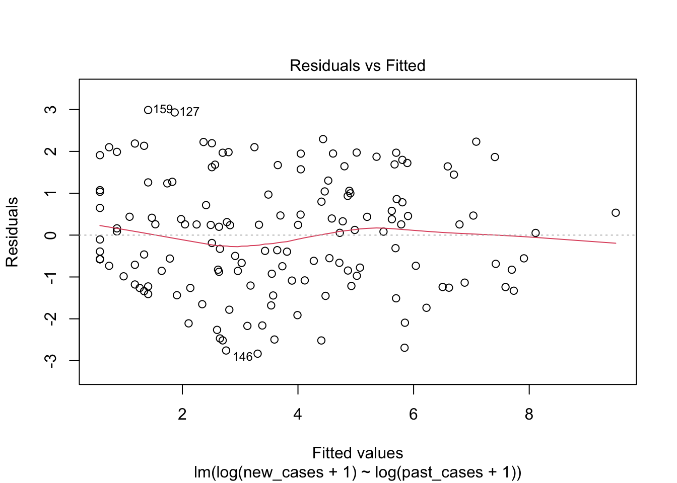
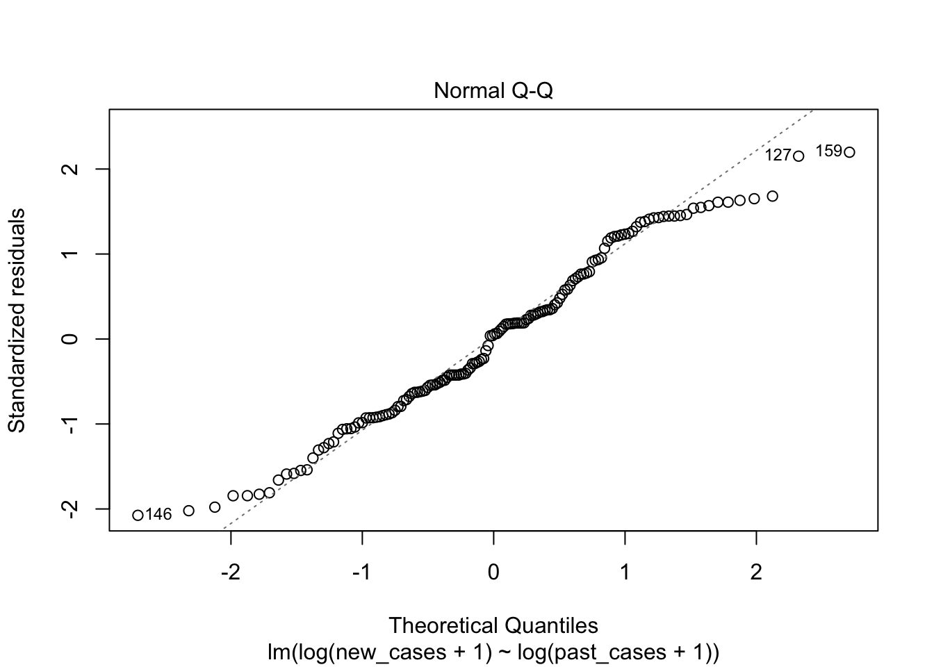
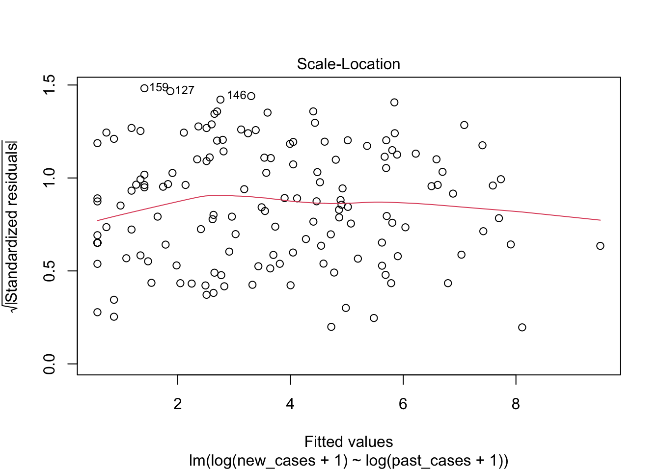
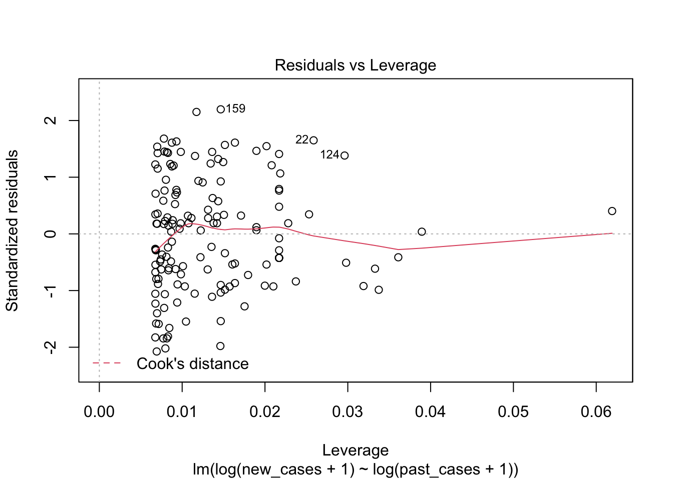
tidy(model_pastonly)## # A tibble: 2 x 5
## term estimate std.error statistic p.value
## <chr> <dbl> <dbl> <dbl> <dbl>
## 1 (Intercept) 0.575 0.202 2.85 5.04e- 3
## 2 log(past_cases + 1) 0.872 0.0478 18.2 1.83e-39tidy(drop1(model_pastonly))## Warning in tidy.anova(drop1(model_pastonly)): The following column names in
## ANOVA output were not recognized or transformed: AIC## # A tibble: 2 x 5
## term df sumsq rss AIC
## <chr> <dbl> <dbl> <dbl> <dbl>
## 1 <none> NA NA 274. 95.2
## 2 log(past_cases + 1) 1 624. 898. 269.So far we learnt to explore our data before fitting models, and then fitting and evaluating models, making transformations if needed. Finally, we learnt to simplify models and drop unnecessary terms. Now we will learn how to use these models to make predictions, and plot them.
Prediction
We will finish our overview of linear models in R by using them for predictions. First, we will fit a new, very complex, model in which the current number of cases of covid19 depends on all variables that we kept on the dataset. We will also include an interaction between gdp per capita and income support, since the effect of support might be greater in poorer countries, for example. We will then do several rounds of drop1() and fitting a simpler model, until we are left only with the variables that are important in explaining variation of new cases across countries.
covid_full_model <- lm(formula = log(new_cases+1) ~ log(past_cases+1) +
                        gdp_per_capita*income_support +
                        stringency_idx +
                        work_close,
                       data=covid_small)
With many variables like this, it will be a lot of work to use drop1() several times, fit simpler models, and repeat. Luckily, R has a function that does that automatically, names step(). As the name indicates, step() does drop1() in steps.
minimal_model <- step(covid_full_model)## Start: AIC=90.71
## log(new_cases + 1) ~ log(past_cases + 1) + gdp_per_capita * income_support +
## stringency_idx + work_close
##
## Df Sum of Sq RSS AIC
## - work_close 3 4.23 239.66 87.339
## <none> 235.44 90.706
## - stringency_idx 1 4.62 240.06 91.581
## - gdp_per_capita:income_support 2 8.64 244.08 92.041
## - log(past_cases + 1) 1 532.18 767.62 263.620
##
## Step: AIC=87.34
## log(new_cases + 1) ~ log(past_cases + 1) + gdp_per_capita + income_support +
## stringency_idx + gdp_per_capita:income_support
##
## Df Sum of Sq RSS AIC
## - stringency_idx 1 1.55 241.22 86.296
## <none> 239.66 87.339
## - gdp_per_capita:income_support 2 8.91 248.58 88.744
## - log(past_cases + 1) 1 560.37 800.03 263.741
##
## Step: AIC=86.3
## log(new_cases + 1) ~ log(past_cases + 1) + gdp_per_capita + income_support +
## gdp_per_capita:income_support
##
## Df Sum of Sq RSS AIC
## <none> 241.22 86.296
## - gdp_per_capita:income_support 2 8.03 249.24 87.140
## - log(past_cases + 1) 1 576.49 817.71 264.976Here, it first found that removing workplace closures improved the model, which we knew already. Then it removed several other predictors in the next steps of drop1(). In the last step, a model including number of past cases and the interaction between income support and gdp per capita was better than any model removing these variables, so we kept them.
Let’s have a look at the chosen model:
plot(minimal_model)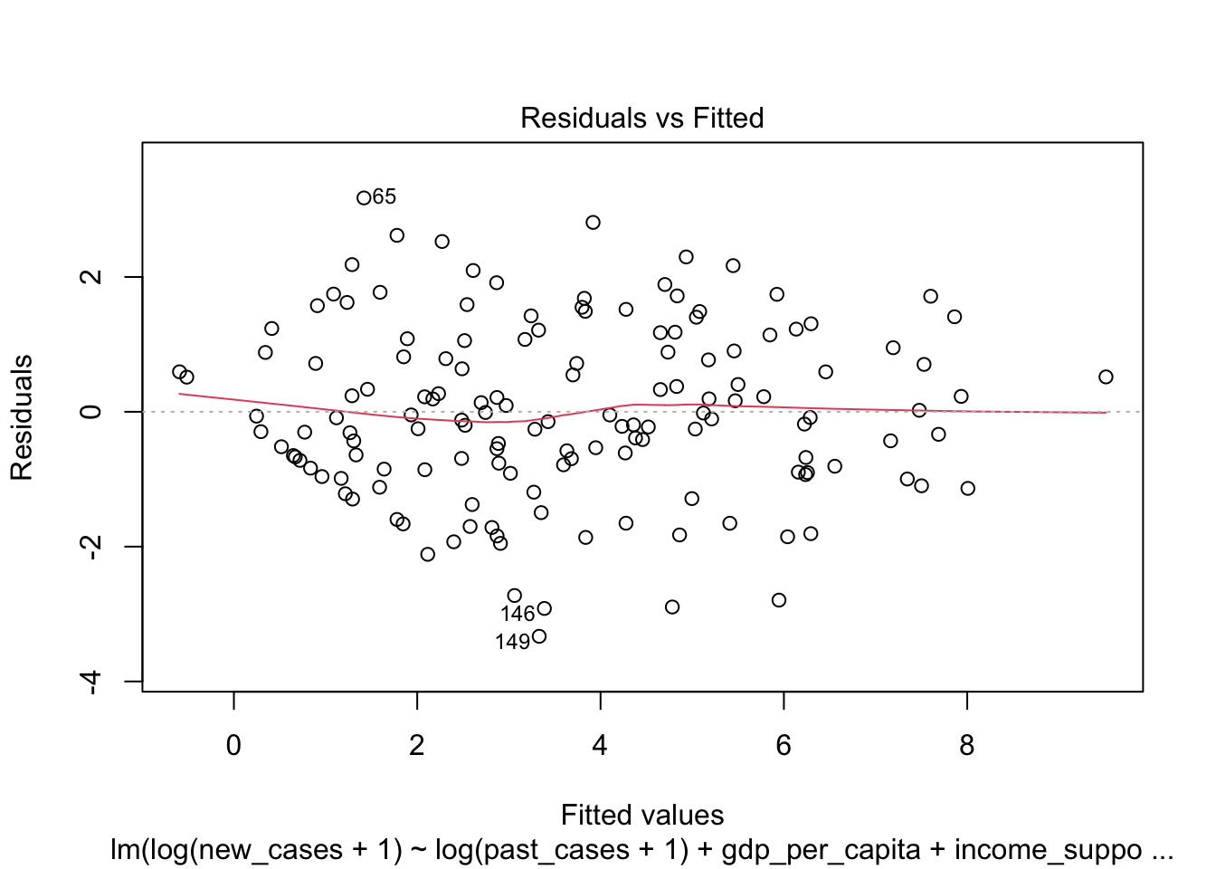
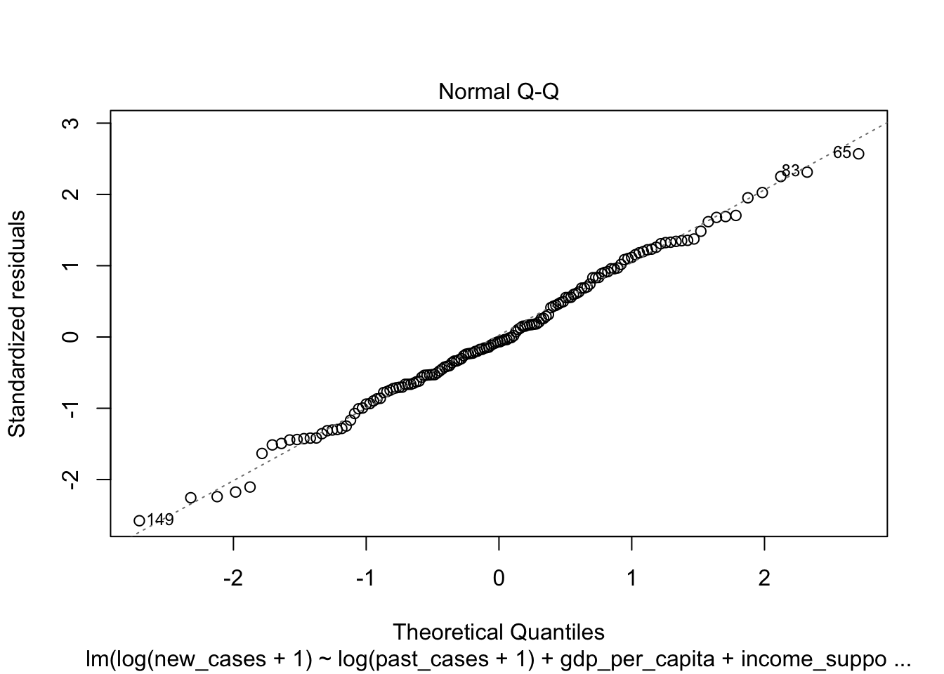
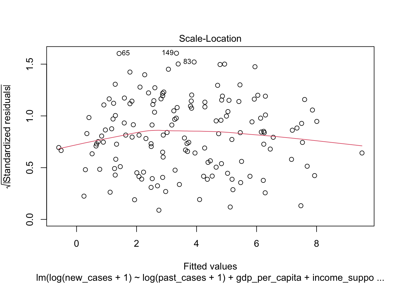
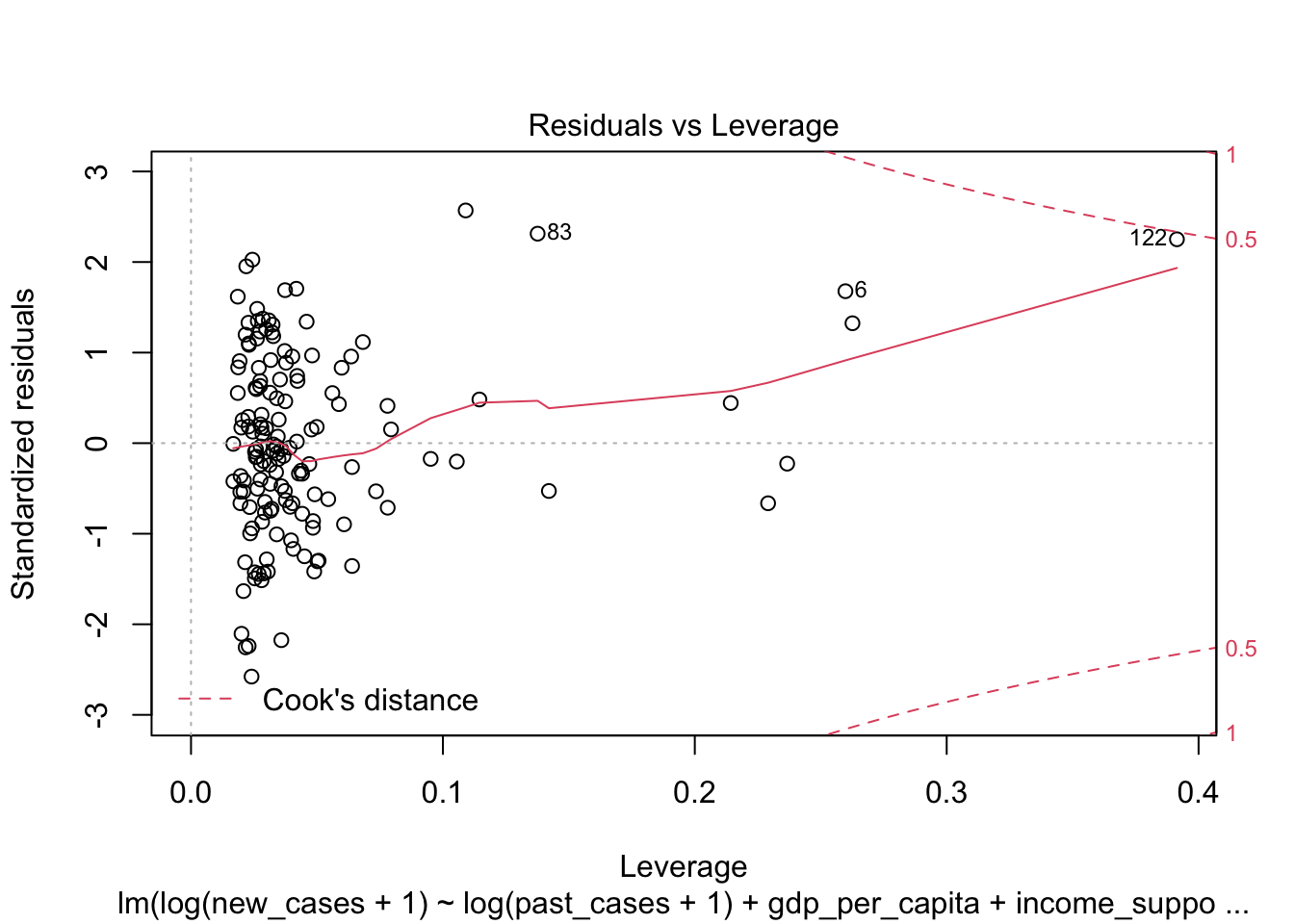
summary(minimal_model)##
## Call:
## lm(formula = log(new_cases + 1) ~ log(past_cases + 1) + gdp_per_capita +
## income_support + gdp_per_capita:income_support, data = covid_small)
##
## Residuals:
## Min 1Q Median 3Q Max
## -3.3306 -0.8396 -0.0870 0.9145 3.1723
##
## Coefficients:
## Estimate Std. Error t value Pr(>|t|)
## (Intercept) 2.715e-01 2.486e-01 1.092 0.27664
## log(past_cases + 1) 9.827e-01 5.353e-02 18.357 < 2e-16 ***
## gdp_per_capita -1.475e-05 6.322e-06 -2.333 0.02108 *
## income_support.L -1.106e+00 3.662e-01 -3.019 0.00301 **
## income_support.Q -2.333e-01 2.929e-01 -0.797 0.42695
## gdp_per_capita:income_support.L 2.350e-05 1.085e-05 2.165 0.03208 *
## gdp_per_capita:income_support.Q -1.414e-06 1.012e-05 -0.140 0.88909
## ---
## Signif. codes: 0 '***' 0.001 '**' 0.01 '*' 0.05 '.' 0.1 ' ' 1
##
## Residual standard error: 1.308 on 141 degrees of freedom
## Multiple R-squared: 0.7314, Adjusted R-squared: 0.72
## F-statistic: 64 on 6 and 141 DF, p-value: < 2.2e-16The summary indicates that the effect of income support alone is mostly linear: the higher the income support, the lower the number of current cases, after accounting for number of past cases. However, the interaction term indicates that if gdp per capita increases, the effect of income support is smaller: income support has a greater effect on poorer countries! It might be hard to understand the model behavior by looking at this table alone, so we will make it easier: let’s use the model to make predictions and then plot these predictions together with the data.
Let’s start by make predictions to compare to the data used to fit the model. We can achieve this with the function predict(). Let’s use predict() to obtain predictions and their associated error:
prediction <- predict(minimal_model, interval = 'prediction')## Warning in predict.lm(minimal_model, interval = "prediction"): predictions on current data refer to _future_ responseshead(prediction)## fit lwr upr
## 1 0.6695544 -2.0094681 3.348577
## 2 4.8131704 2.1868262 7.439515
## 3 0.7722633 -1.8490491 3.393576
## 4 2.1703236 -0.5161315 4.856779
## 6 4.7016893 1.7994289 7.603950
## 7 4.6524578 2.0418860 7.263030Now we need to remember that we log-transformed the response variable (number of new covid19 cases) before fitting the model, so we need to do the inverse operation here so our prediction is in the original scale. The inverse function of \(log(x+1)\) is \(exp(x)-1\).
prediction_df = as.data.frame(exp(prediction)-1)

head(prediction_df)
## fit lwr upr
## 1 0.9533668 -0.8659400 27.46220
## 2 122.1213442 7.9068999 1700.92386
## 3 1.1646600 -0.8426132 28.77222
## 4 7.7611190 -0.4031751 127.60925
## 6 109.1330581 5.0461935 2005.10358
## 7 103.8423464 6.7051274 1425.57182We can join this data.frame to the data used in the model fit by binding columns with cbind()
data_plus_pred = cbind(prediction_df, covid_small)

head(data_plus_pred)
## fit lwr upr country_name
## 1 0.9533668 -0.8659400 27.46220 Aruba
## 2 122.1213442 7.9068999 1700.92386 Afghanistan
## 3 1.1646600 -0.8426132 28.77222 Angola
## 4 7.7611190 -0.4031751 127.60925 Albania
## 6 109.1330581 5.0461935 2005.10358 United Arab Emirates
## 7 103.8423464 6.7051274 1425.57182 Argentina
## world_region new_cases past_cases gdp_per_capita
## 1 Latin America and the Caribbean 0.0 1.4 35973.781
## 2 Asia and the Pacific 400.0 52.6 1803.987
## 3 Africa 0.6 0.0 5819.495
## 4 Europe 9.6 15.6 11803.431
## 6 West Asia 726.6 401.0 67293.483
## 7 Latin America and the Caribbean 338.0 91.4 18933.907
## work_close income_support stringency_idx
## 1 require most none 83.46
## 2 require most none 76.33
## 3 require some none 86.77
## 4 require some more than 50% 88.36
## 6 require some none 86.77
## 7 require some less than 50% 87.57How good was our prediction for Panama, Brazil and the USA, for example?
countries = c('Panama', 'Brazil', 'United States')

data_plus_pred[data_plus_pred$country_name %in% countries, c('lwr','fit','upr','new_cases','country_name')]
## lwr fit upr new_cases country_name
## 22 141.15920 1999.9313 28162.677 11104.8 Brazil
## 113 12.25588 182.4582 2538.018 164.0 Panama
## 153 923.24146 13542.7191 198466.971 22719.6 United StatesThe number of cases is within the prediction interval, but the average is one order of magnitude wrong for Brazil.
We can also make predictions based on new data. This is useful to make nice plots including the data and model predictions, for example. Let’s try it out. First, we will figure out what is the range of the data we will plot.
summary(covid_small$income_support)## none less than 50% more than 50%
## 60 56 32summary(covid_small$past_cases)## Min. 1st Qu. Median Mean 3rd Qu. Max.
## 0.0 3.9 28.0 501.0 161.6 27620.8summary(covid_small$gdp_per_capita)## Min. 1st Qu. Median Mean 3rd Qu. Max.
## 702.2 5288.6 13567.3 20588.0 31654.4 116935.6So we need to make predictions across the range of 0-27620 of new daily cases, for the 3 levels of income support. It would be hard to do that for all of the range of gdp per capita, so we will make predictions for two kinds of countries: a poor country with gdp per capita of US$ 5,000 per year and a rich country with gdp per capita of US$ 50,000 per year.
We need create a data.frame with all possible combinations for the values from all three variables, which we can do with the function expand.grid(). expand.grid() creates a new data frame with all possible combinations of the vectors provided.
values_past_cases <- seq(from = 0, to=27620, length.out = 1000)
values_income <- levels(covid_small$income_support)

values_gdp <- c(5000, 50000)

new_data <- expand.grid(values_past_cases, values_income, values_gdp)

head(new_data)
## Var1 Var2 Var3
## 1 0.00000 none 5000
## 2 27.64765 none 5000
## 3 55.29530 none 5000
## 4 82.94294 none 5000
## 5 110.59059 none 5000
## 6 138.23824 none 5000A side effect of expand.grid() is that ordered factors loose their order, so we need to use the function factor() to put the correct order back. This is important for plotting, since ggplot will automatically recognize the order and use an appropriate color scale.
new_data$Var2 <- factor(new_data$Var2,
                       levels = levels(covid_small$income_support),
                       ordered = T)
Now we have to rename our data.frame columns to match the model parameters, and to transform income support into a factor as it was originally.
colnames(new_data) <- c('past_cases', 'income_support','gdp_per_capita')

head(new_data)
## past_cases income_support gdp_per_capita
## 1 0.00000 none 5000
## 2 27.64765 none 5000
## 3 55.29530 none 5000
## 4 82.94294 none 5000
## 5 110.59059 none 5000
## 6 138.23824 none 5000Now that we have the data.fame with new data, we can use it to predict. Let’s make the predictions and add them as new columns to the new_data data.frame after transforming back to the original scale
prediction <- predict(minimal_model, newdata = new_data, interval = 'prediction')
prediction <- exp(prediction) - 1

new_data <- cbind(new_data, prediction)

head(new_data)
## past_cases income_support gdp_per_capita fit lwr upr
## 1 0.00000 none 5000 1.222061 -0.8385641 29.58525
## 2 27.64765 none 5000 59.067018 3.3928636 820.34273
## 3 55.29530 none 5000 115.665759 7.4938184 1601.44764
## 4 82.94294 none 5000 171.764132 11.5332004 2380.47037
## 5 110.59059 none 5000 227.537685 15.5303396 3158.61287
## 6 138.23824 none 5000 283.070160 19.4950177 3936.34013Before plotting, let’s add a new column that will say if a country is rich or poor depending on the gdp per capita. We will call countries above 30,000 USD as rich and those below this as poor by using the function ifelse(). This function works similar to an if{} else{} statement, but it is a much shorter version for vectors. The function below means that the column country_type will have a value of rich if the country has a gdp per capita above 30000, and poor if not.
new_data$country_type <- ifelse(new_data$gdp_per_capita > 30000,
                               'rich',
                               'poor')
We will do the same for our real data.
covid_small$country_type = ifelse(covid_small$gdp_per_capita > 30000,
                               'rich',
                               'poor')
Now we can use ggplot to plot the data and the predictions. Let’s start with the predictions. We will plot rich and poor countries as facets, income support as colors, past cases in the X axis and new cases in the Y axis as a line. Since we are using a line and not points, we need also to use the group aesthetics, to tell which points will be part of the same line
p <- ggplot(new_data) +
  geom_line(aes(x = past_cases,
                 y = fit,
                 color = income_support,
                 group = income_support)) +
  facet_wrap(~country_type)

p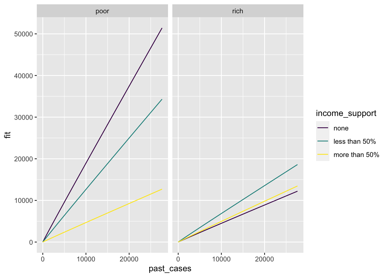
Looking at the prediction alone, it seems that for poor countries the higher the income support, the lower the increase in number of new cases during the last month. The effect is smaller for rich countries.
Now let’s add the real data. Remember that since we assigned our plot to the variable p, we can add a new plot layer by adding a geom_ to p. Let’s add points, and indicate the the data comes from covid_small.
p <- p +
  geom_point(aes(x = past_cases,
                 y = new_cases,
                 color = income_support,
                 group = income_support),
             data = covid_small)

p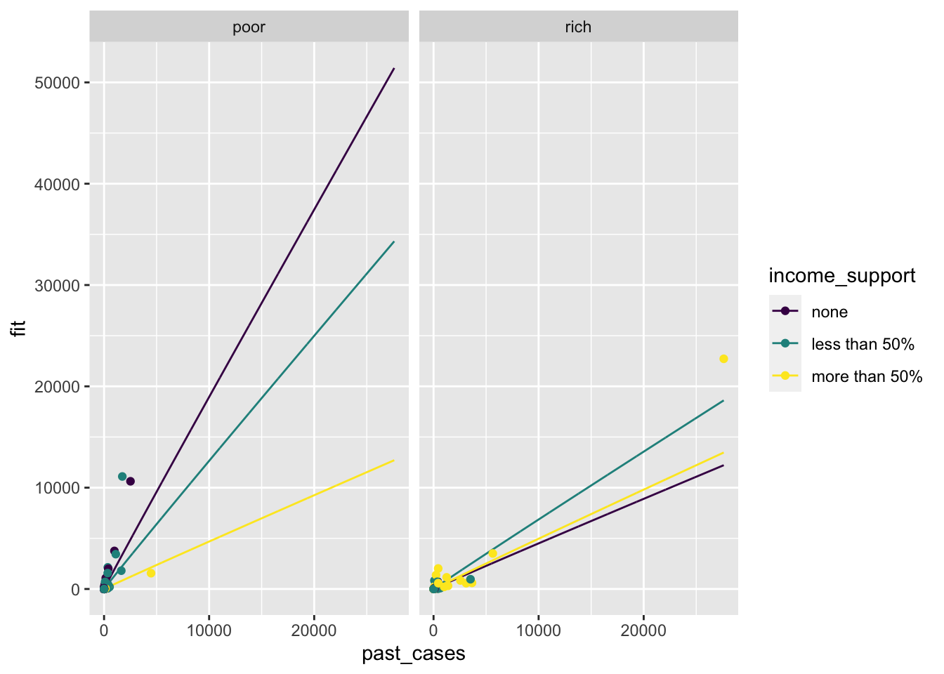
Oops, it is hard to visualize the data. Let’s transform scales to a log1p scale for better visualizing:
p <- p +
  scale_x_continuous(trans = 'log1p', breaks = 10^(0:5)) +
  scale_y_continuous(trans = 'log1p', breaks = 10^(0:5))

p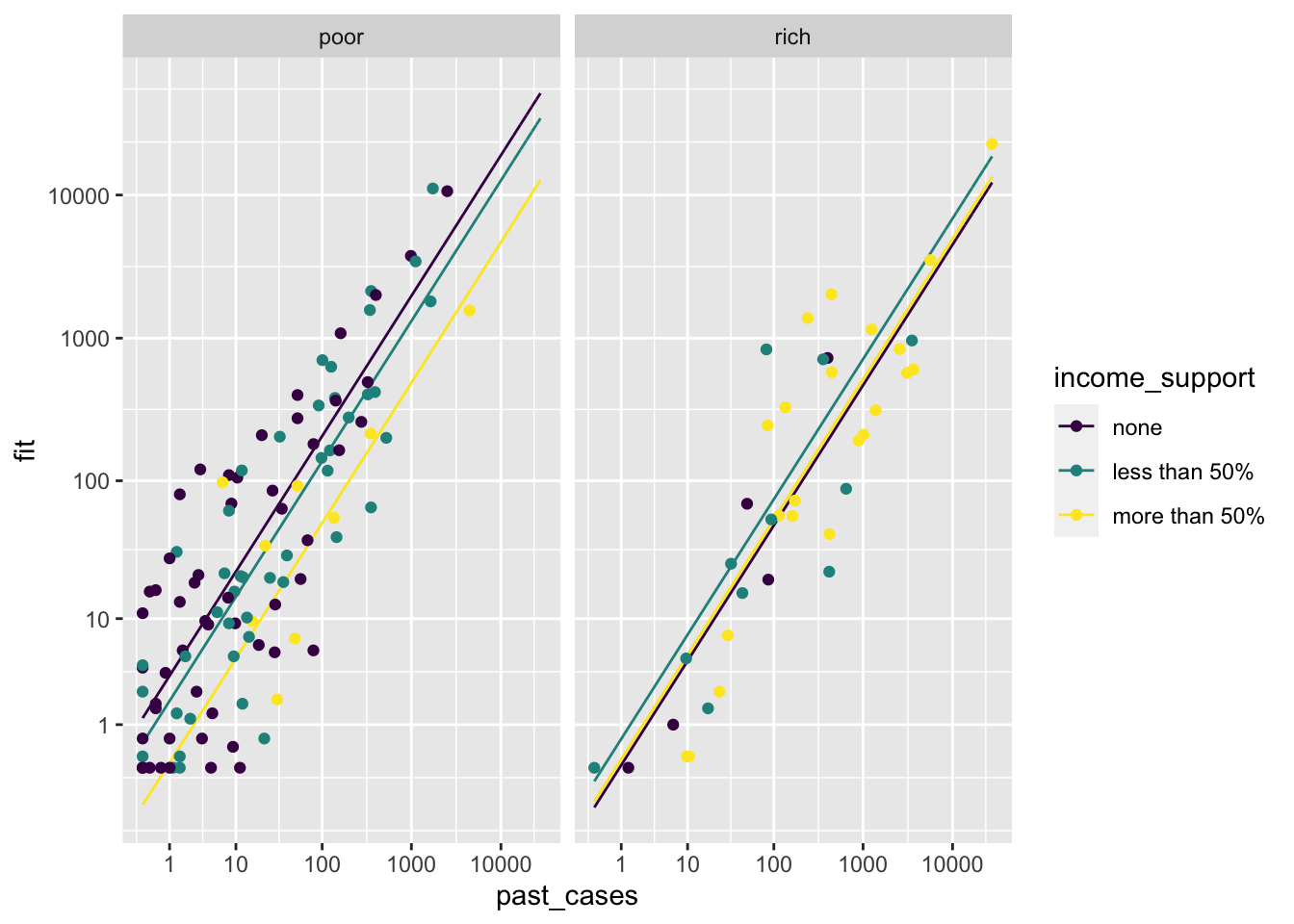
With this plot, a few things stand out:
There is quite a lot of variation in the degree of income support across countries, which might have played a role in the power that we had to detect a relationship.
There is some degree of correlation between gdp per capita and income support: a larger share of rich countries seem to have done it, when compared to poor countries. That said, there is variation in both classes.
We should be careful when interpreting results. It does not mean that international travel control does not work, for example. Since most countries implemented some degree of control, it might be the case that we just do not have enough variation to test whether it works or not. This is one of the limitations of observational data in comparison to experiments!
Finally, we can embellish the plot with nice labels and a nice theme. We will also add a 1:1 dashed line which will indicate which countries increased and which decreased cases with geom_abline(). Points below the dashed line decreased in cases in the last 30 days, and it is pretty clear that income support brings more points below the line:
p +
  theme_minimal() +
  labs(y = 'Average new cases in the past 5 days',
       x = 'Average new cases a month ago',
       title = 'Growth of COVID19 across countries',
       subtitle = 'Income decreases cases of COVID19') +
  geom_abline(intercept = 0,slope = 1,linetype='dashed') +
  coord_equal()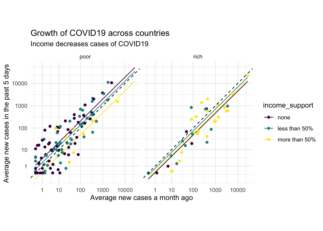
This concludes our tutorial on linear models. There is a lot more that can be done in R for more complex models, but they all use similar functions to the ones we used here. To learn more, check the following:
Generalized linear models: function
glm.Time Series: several packages.
Mixed models: several packages
Linear models accounting for phylogeny: several packages
Bayesian models: rstanarm for an easy interface similar to the one we used here.
Clustering and ordination
R is also a great tool to work with multivariate data, which we typically find in community ecology, for example. A common analysis with this kind of data is clustering and ordination. In our context here, we can ask ourselves how countries differ overall in the kind of interventions that they have taken against covid19, and whether countries in the same region tend to be more similar. We will use a method known as ‘nonmetric multidimensional scaling’ to visualize that, and an analysis of variance based on permutation (PERMANOVA) to test if kinds of measures differ by world region.
Let’s start by reading a new data.frame including only columns for country interventions against covid19, world regions and country names. This is a smaller version of the full data, in which we removed interventions with too much missing data
covid_interventions <- read.csv('covid_interventions_2020-05-16.csv', row.names = 1)
head(covid_interventions)
## world_region country_name C1_School.closing
## 1 Latin America and the Caribbean Aruba 3
## 2 Asia and the Pacific Afghanistan 3
## 3 Africa Angola 3
## 4 Europe Albania 3
## 5 Europe Andorra 3
## 6 West Asia United Arab Emirates 3
## C1_Flag C2_Workplace.closing C3_Cancel.public.events C3_Flag
## 1 1 3 2 1
## 2 1 3 2 1
## 3 1 2 2 1
## 4 1 2 2 1
## 5 1 2 1 1
## 6 1 2 2 1
## C4_Restrictions.on.gatherings C5_Close.public.transport
## 1 4 0
## 2 4 2
## 3 4 1
## 4 4 2
## 5 0 1
## 6 4 1
## C6_Stay.at.home.requirements C7_Restrictions.on.internal.movement
## 1 2 2
## 2 2 2
## 3 2 2
## 4 2 2
## 5 1 0
## 6 2 1
## C8_International.travel.controls E1_Income.support E2_Debt.contract.relief
## 1 3 0 2
## 2 1 0 0
## 3 4 0 2
## 4 4 2 1
## 5 3 2 0
## 6 4 0 2
## H1_Public.information.campaigns H1_Flag H2_Testing.policy H3_Contact.tracing
## 1 2 1 1 0
## 2 2 1 1 1
## 3 1 1 2 0
## 4 2 1 2 1
## 5 2 1 3 1
## 6 2 1 3 2
## H4_Emergency.investment.in.healthcare H5_Investment.in.vaccines
## 1 0 0
## 2 0 0
## 3 0 0
## 4 0 0
## 5 0 0
## 6 0 0The first step to do an ordination is to transform this table with several variables a summary with how different each country is from each other overall. In ecology, this would be the \(\beta\) diversity, but here we will calculate Euclidean distances. This can be done with the R function dist(). For ecology, the package ecodist has functions to calculate several kinds of distance metrics.
The differences between all countries (ignoring columns with country names and regions) are:
intervention_differences <- dist(covid_interventions[,-c(1,2)])If we look at this object now, we find that it is an object of the class dist, that records the pairwise distances between all 147 countries (10731 distances total)
str(intervention_differences)## 'dist' num [1:10731] 3.61 2.24 3.61 6.08 3.46 ...
## - attr(*, "Size")= int 147
## - attr(*, "Labels")= chr [1:147] "1" "2" "3" "4" ...
## - attr(*, "Diag")= logi FALSE
## - attr(*, "Upper")= logi FALSE
## - attr(*, "method")= chr "euclidean"
## - attr(*, "call")= language dist(x = covid_interventions[, -c(1, 2)])We will now use nonmetric multidimensional scaling (NMDS) to reduce this distance matrix of 147$$147 to only 2 dimensions, that we humans can look at in a graph. NMDS will attempt to represent the distances betwen all points in these two dimensions as well as possible.
The R package vegan() contains several functions to work with multivariate data, including one to do MDS. Let’s load the package first and remembet to install it with install.packages('vegan') in case you do not have it in your library already.
library(vegan)## Loading required package: permute## Loading required package: lattice## This is vegan 2.5-6The function to do NMDS is metaMDS:
mds <- metaMDS(intervention_differences)## Run 0 stress 0.2121924
## Run 1 stress 0.2103559
## ... New best solution
## ... Procrustes: rmse 0.03011934 max resid 0.1736358
## Run 2 stress 0.2109125
## Run 3 stress 0.2127114
## Run 4 stress 0.210966
## Run 5 stress 0.2109142
## Run 6 stress 0.210914
## Run 7 stress 0.2101792
## ... New best solution
## ... Procrustes: rmse 0.01025439 max resid 0.1061251
## Run 8 stress 0.2169023
## Run 9 stress 0.2208988
## Run 10 stress 0.214967
## Run 11 stress 0.2190474
## Run 12 stress 0.2110621
## Run 13 stress 0.2149936
## Run 14 stress 0.2203084
## Run 15 stress 0.2203263
## Run 16 stress 0.2128381
## Run 17 stress 0.2110632
## Run 18 stress 0.210858
## Run 19 stress 0.2115449
## Run 20 stress 0.2209754
## *** No convergence -- monoMDS stopping criteria:
## 20: stress ratio > sratmaxWe can use plot to visualize the results now:
plot(mds)## species scores not available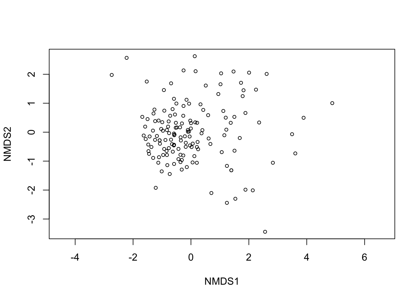
If we want to color by world region, we can combine the points from the mds result with our column for country names and regions. The object mds, to which we assigned MDS results, holds the data frame with points under a slot named points. So here, with mds$points we can retrieve it.
mds_result <- cbind(mds$points, covid_interventions)

head(mds_result)
## MDS1 MDS2 world_region country_name
## 1 -1.2609993 0.7811568 Latin America and the Caribbean Aruba
## 2 -1.2163974 -1.9220767 Asia and the Pacific Afghanistan
## 3 -0.7699213 0.3721168 Africa Angola
## 4 -0.5776075 -0.1048845 Europe Albania
## 5 3.6053812 -0.7335618 Europe Andorra
## 6 -0.5520690 0.6102937 West Asia United Arab Emirates
## C1_School.closing C1_Flag C2_Workplace.closing C3_Cancel.public.events
## 1 3 1 3 2
## 2 3 1 3 2
## 3 3 1 2 2
## 4 3 1 2 2
## 5 3 1 2 1
## 6 3 1 2 2
## C3_Flag C4_Restrictions.on.gatherings C5_Close.public.transport
## 1 1 4 0
## 2 1 4 2
## 3 1 4 1
## 4 1 4 2
## 5 1 0 1
## 6 1 4 1
## C6_Stay.at.home.requirements C7_Restrictions.on.internal.movement
## 1 2 2
## 2 2 2
## 3 2 2
## 4 2 2
## 5 1 0
## 6 2 1
## C8_International.travel.controls E1_Income.support E2_Debt.contract.relief
## 1 3 0 2
## 2 1 0 0
## 3 4 0 2
## 4 4 2 1
## 5 3 2 0
## 6 4 0 2
## H1_Public.information.campaigns H1_Flag H2_Testing.policy H3_Contact.tracing
## 1 2 1 1 0
## 2 2 1 1 1
## 3 1 1 2 0
## 4 2 1 2 1
## 5 2 1 3 1
## 6 2 1 3 2
## H4_Emergency.investment.in.healthcare H5_Investment.in.vaccines
## 1 0 0
## 2 0 0
## 3 0 0
## 4 0 0
## 5 0 0
## 6 0 0Now we can use ggplot to plot the points and color by region:
ggplot(mds_result) +
  geom_point(aes(x = MDS1,
                 y = MDS2,
                 color = world_region))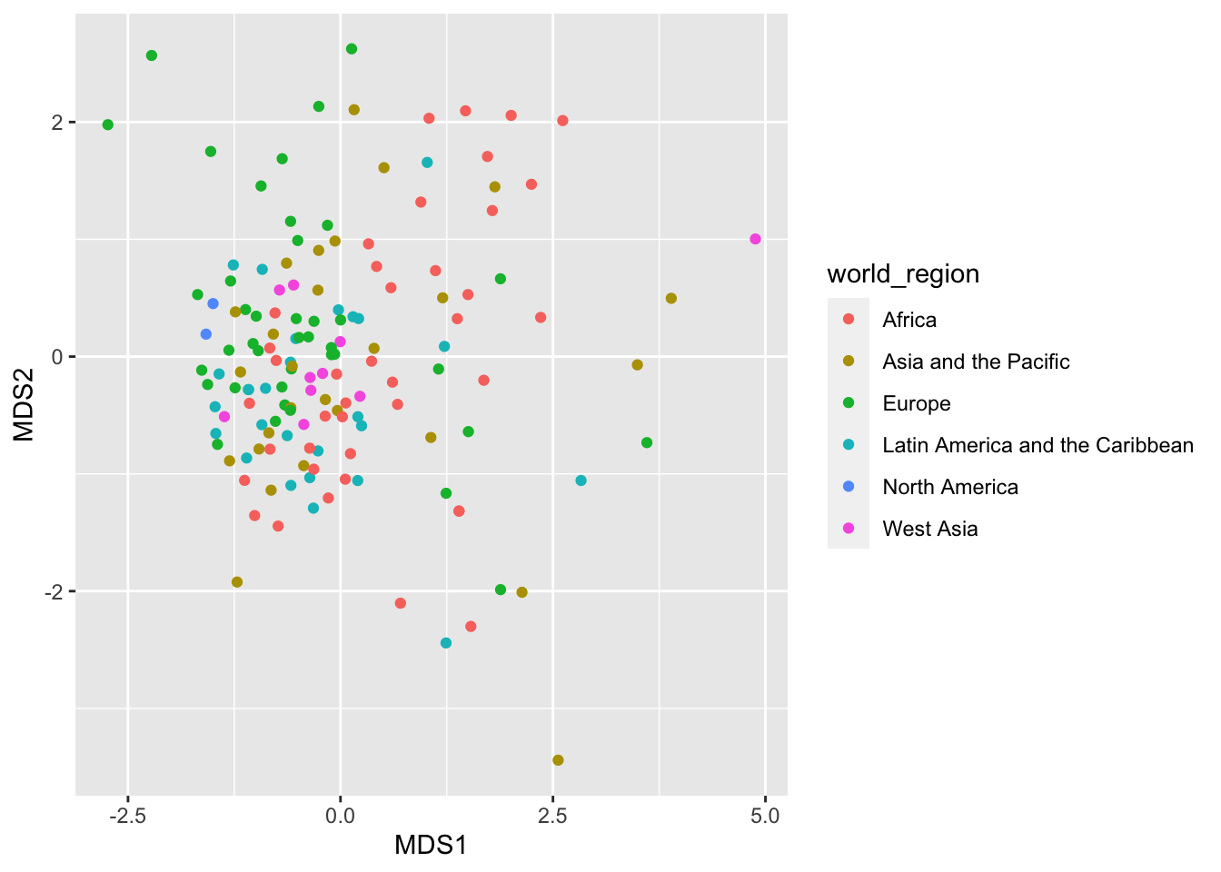
With ggplot, we can also add ellipses surrounding the points for each region. We use the aesthetics group because stat_ellipse() needs to know how to group the points. We also moved the aesthetics up to the ggplot() function so it is inherited by both geom_point() and stat_ellipse().
ggplot(mds_result, aes(x = MDS1, y = MDS2, color = world_region, group = world_region)) +
  geom_point() +
  stat_ellipse() +
  scale_color_brewer(type='qual')
## Too few points to calculate an ellipse## Warning: Removed 1 row(s) containing missing values (geom_path).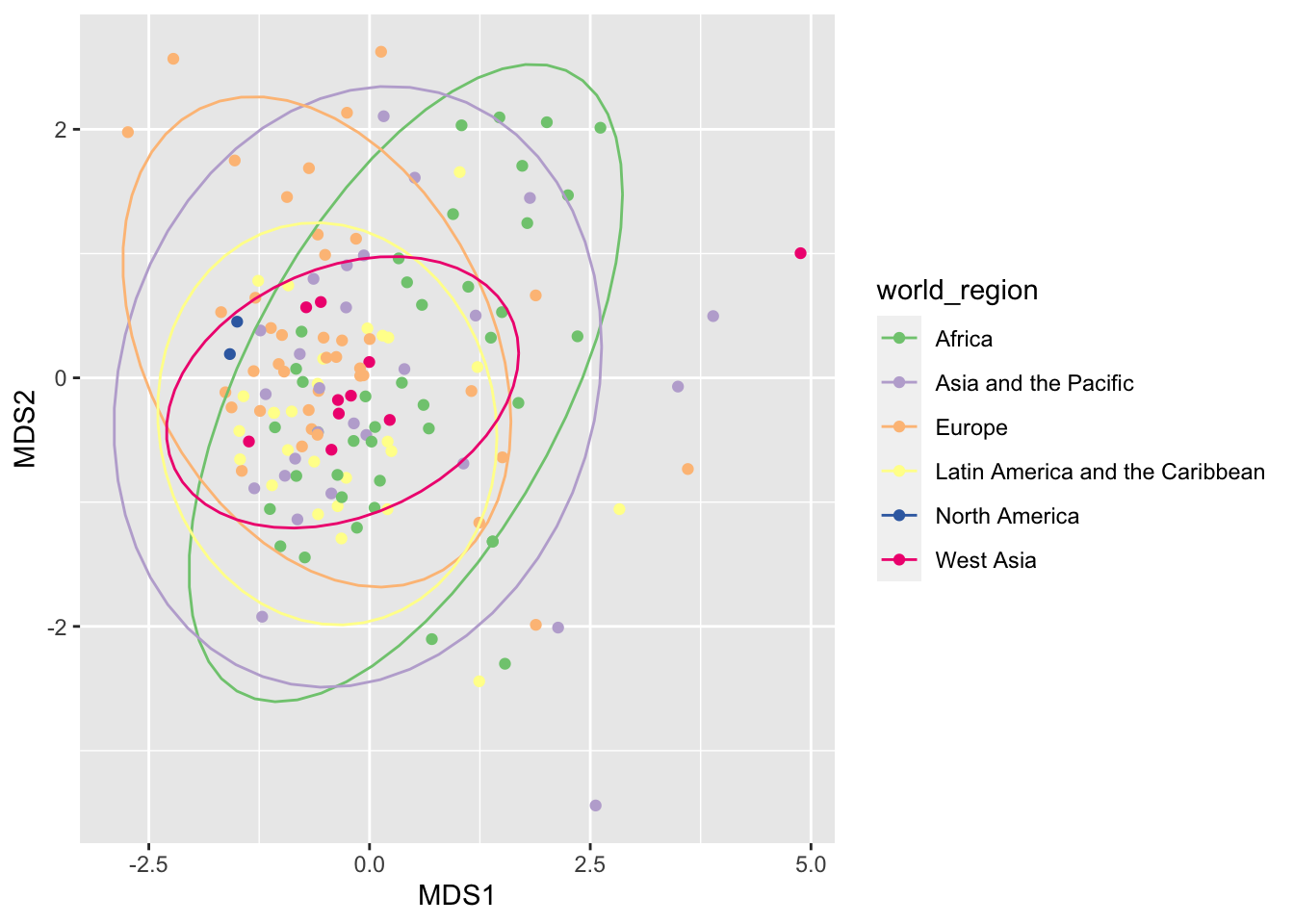
We got a warning because North America only has two countries and therefore it is not possible to draw an ellipse.
Maybe there is some difference between countries, but it is not clear. Let’s test whether this is the case with with a permutational ANOVA. By using the distances between countries as our response and world regions as the predictor, we want to know whether world regions differ significantly in the interventions used against covid19. The function to do this analysis is adonis2 in the package vegan, and it uses a formula similar to linear models:
adonis2(intervention_differences ~ world_region, data = covid_interventions)## Permutation test for adonis under reduced model
## Terms added sequentially (first to last)
## Permutation: free
## Number of permutations: 999
##
## adonis2(formula = intervention_differences ~ world_region, data = covid_interventions)
## Df SumOfSqs R2 F Pr(>F)
## world_region 5 87.68 0.08315 2.5576 0.001 ***
## Residual 141 966.75 0.91685
## Total 146 1054.44 1.00000
## ---
## Signif. codes: 0 '***' 0.001 '**' 0.01 '*' 0.05 '.' 0.1 ' ' 1It seems there is a difference between regions!
To summarize, we used linear models to find that there is a difference between regions in the number of new covid19 in the last few days. With a PERMANOVA, we found also that there is a difference in the interventions that countries in different regions attempted.
With a more complex model including other variables beyond region, we found that the number of new covid19 cases can be well explained by the number of past cases, and that governments providing some sort of income to their population were more sucessful in reducing the number of new cases. This effect was stronger in poorer countries.
To find out more about multivariate analyses and methods for ordination applied to ecology, checkout the page linked here.
To do
As an exercise, try to select different columns from the full dataset
covid_dataand use linear models to find the effect of other variables (for example, population age or density, prevalence of diabetes, etc) on the number of cases. You can also try to change the response variable to the total number of cases instead of the daily cases.Try to apply either linear models or ordination to another dataset. If you have ecology data, come to office hours and we can work together on how to use ordination with dissimilarity metrics that are appropriate to ecology.
Appendix: Producing the dataset
Here we show how the dataset that we used in this tutorial was produced. It is the result of cleaning and merging three sources: a table including country-level covid19 cases and country demographic data, another table with country responses to covid19, and a table that includes information about countries, including in which continent they are in.
After merging this data in a single table, we saved it as the csv file that we used today.
Loading and cleaning datasets
Let’s start by downloading the data. The covid19 data in Our World in Data is updated daily, and we can get the most recent table directly from the link https://covid.ourworldindata.org/data/owid-covid-data.csv
In the previous tutorials, we have loaded datasets located in our computer, and we could in theory use a web browser to download the table first, and then load it to R. However, R allows us to load a file directly from the web if we provide a URL (i. e. a web address). This table is in the CSV format (i. e. comma-separated values), so we will use the function read.csv() to read it.
country_covid <- read.csv('https://covid.ourworldindata.org/data/owid-covid-data.csv')

head(country_covid)
## iso_code continent location date total_cases new_cases total_deaths
## 1 ABW North America Aruba 2020-03-13 2 2 0
## 2 ABW North America Aruba 2020-03-20 4 2 0
## 3 ABW North America Aruba 2020-03-24 12 8 0
## 4 ABW North America Aruba 2020-03-25 17 5 0
## 5 ABW North America Aruba 2020-03-26 19 2 0
## 6 ABW North America Aruba 2020-03-27 28 9 0
## new_deaths total_cases_per_million new_cases_per_million
## 1 0 18.733 18.733
## 2 0 37.465 18.733
## 3 0 112.395 74.930
## 4 0 159.227 46.831
## 5 0 177.959 18.733
## 6 0 262.256 84.296
## total_deaths_per_million new_deaths_per_million new_tests total_tests
## 1 0 0 NA NA
## 2 0 0 NA NA
## 3 0 0 NA NA
## 4 0 0 NA NA
## 5 0 0 NA NA
## 6 0 0 NA NA
## total_tests_per_thousand new_tests_per_thousand new_tests_smoothed
## 1 NA NA NA
## 2 NA NA NA
## 3 NA NA NA
## 4 NA NA NA
## 5 NA NA NA
## 6 NA NA NA
## new_tests_smoothed_per_thousand tests_units stringency_index population
## 1 NA 0.00 106766
## 2 NA 33.33 106766
## 3 NA 44.44 106766
## 4 NA 44.44 106766
## 5 NA 44.44 106766
## 6 NA 44.44 106766
## population_density median_age aged_65_older aged_70_older gdp_per_capita
## 1 584.8 41.2 13.085 7.452 35973.78
## 2 584.8 41.2 13.085 7.452 35973.78
## 3 584.8 41.2 13.085 7.452 35973.78
## 4 584.8 41.2 13.085 7.452 35973.78
## 5 584.8 41.2 13.085 7.452 35973.78
## 6 584.8 41.2 13.085 7.452 35973.78
## extreme_poverty cardiovasc_death_rate diabetes_prevalence female_smokers
## 1 NA NA 11.62 NA
## 2 NA NA 11.62 NA
## 3 NA NA 11.62 NA
## 4 NA NA 11.62 NA
## 5 NA NA 11.62 NA
## 6 NA NA 11.62 NA
## male_smokers handwashing_facilities hospital_beds_per_thousand
## 1 NA NA NA
## 2 NA NA NA
## 3 NA NA NA
## 4 NA NA NA
## 5 NA NA NA
## 6 NA NA NA
## life_expectancy
## 1 76.29
## 2 76.29
## 3 76.29
## 4 76.29
## 5 76.29
## 6 76.29This dataset records, for each country and each date, a series of statistics on covid19 as well together with several other statistics about the country (such as population, age structure, etc). A full explanation of the dataset can be found in this github repository and an explanation of the fields included can be found here, which is copied below:
| Column | Description | Source |
|---|---|---|
iso_code |
ISO 3166-1 alpha-3 – three-letter country codes | International Organization for Standardization |
location |
Geographical location | Our World in Data |
date |
Date of observation | Our World in Data |
total_cases |
Total confirmed cases of COVID-19 | European Centre for Disease Prevention and Control |
new_cases |
New confirmed cases of COVID-19 | European Centre for Disease Prevention and Control |
total_deaths |
Total deaths attributed to COVID-19 | European Centre for Disease Prevention and Control |
new_deaths |
New deaths attributed to COVID-19 | European Centre for Disease Prevention and Control |
total_cases_per_million |
Total confirmed cases of COVID-19 per 1,000,000 people | European Centre for Disease Prevention and Control |
new_cases_per_million |
New confirmed cases of COVID-19 per 1,000,000 people | European Centre for Disease Prevention and Control |
total_deaths_per_million |
Total deaths attributed to COVID-19 per 1,000,000 people | European Centre for Disease Prevention and Control |
new_deaths_per_million |
New deaths attributed to COVID-19 per 1,000,000 people | European Centre for Disease Prevention and Control |
total_tests |
Total tests for COVID-19 | European Centre for Disease Prevention and Control |
new_tests |
New tests for COVID-19 | European Centre for Disease Prevention and Control |
total_tests_per_thousand |
Total tests for COVID-19 per 1,000 people | National government reports |
new_tests_per_thousand |
New tests for COVID-19 per 1,000 people | National government reports |
tests_units |
Units used by the location to report its testing data | National government reports |
population |
Population in 2020 | United Nations, Department of Economic and Social Affairs, Population Division, World Population Prospects: The 2019 Revision |
population_density |
Number of people divided by land area, measured in square kilometers, most recent year available | World Bank – World Development Indicators, sourced from Food and Agriculture Organization and World Bank estimates |
median_age |
Median age of the population, UN projection for 2020 | UN Population Division, World Population Prospects, 2017 Revision |
aged_65_older |
Share of the population that is 65 years and older, most recent year available | World Bank – World Development Indicators, based on age/sex distributions of United Nations Population Division’s World Population Prospects: 2017 Revision |
aged_70_older |
Share of the population that is 70 years and older in 2015 | United Nations, Department of Economic and Social Affairs, Population Division (2017), World Population Prospects: The 2017 Revision |
gdp_per_capita |
Gross domestic product at purchasing power parity (constant 2011 international dollars), most recent year available | World Bank – World Development Indicators, source from World Bank, International Comparison Program database |
extreme_poverty |
Share of the population living in extreme poverty, most recent year available since 2010 | World Bank – World Development Indicators, sourced from World Bank Development Research Group |
cvd_death_rate |
Death rate from cardiovascular disease in 2017 | Global Burden of Disease Collaborative Network, Global Burden of Disease Study 2017 Results |
diabetes_prevalence |
Diabetes prevalence (% of population aged 20 to 79) in 2017 | World Bank – World Development Indicators, sourced from International Diabetes Federation, Diabetes Atlas |
female_smokers |
Share of women who smoke, most recent year available | World Bank – World Development Indicators, sourced from World Health Organization, Global Health Observatory Data Repository |
male_smokers |
Share of men who smoke, most recent year available | World Bank – World Development Indicators, sourced from World Health Organization, Global Health Observatory Data Repository |
handwashing_facilities |
Share of the population with basic handwashing facilities on premises, most recent year available | United Nations Statistics Division |
hospital_beds_per_100k |
Hospital beds per 100,000 people, most recent year available since 2010 | OECD, Eurostat, World Bank, national government records and other sources |
Since we are interested in understanding whether government responses work, we have to join this dataset to another one including several responses of governments to covid19. The link to this second dataset can also be found in the Our World in Data web page, which is this one: https://raw.githubusercontent.com/OxCGRT/covid-policy-tracker/master/data/OxCGRT_latest.csv. Again, we will use read.csv() to load the dataset to a table:
country_response <- read.csv('https://raw.githubusercontent.com/OxCGRT/covid-policy-tracker/master/data/OxCGRT_latest.csv')

head(country_response)
## CountryName CountryCode Date C1_School.closing C1_Flag
## 1 Aruba ABW 20200101 0 NA
## 2 Aruba ABW 20200102 0 NA
## 3 Aruba ABW 20200103 0 NA
## 4 Aruba ABW 20200104 0 NA
## 5 Aruba ABW 20200105 0 NA
## 6 Aruba ABW 20200106 0 NA
## C2_Workplace.closing C2_Flag C3_Cancel.public.events C3_Flag
## 1 0 NA 0 NA
## 2 0 NA 0 NA
## 3 0 NA 0 NA
## 4 0 NA 0 NA
## 5 0 NA 0 NA
## 6 0 NA 0 NA
## C4_Restrictions.on.gatherings C4_Flag C5_Close.public.transport C5_Flag
## 1 0 NA 0 NA
## 2 0 NA 0 NA
## 3 0 NA 0 NA
## 4 0 NA 0 NA
## 5 0 NA 0 NA
## 6 0 NA 0 NA
## C6_Stay.at.home.requirements C6_Flag C7_Restrictions.on.internal.movement
## 1 0 NA 0
## 2 0 NA 0
## 3 0 NA 0
## 4 0 NA 0
## 5 0 NA 0
## 6 0 NA 0
## C7_Flag C8_International.travel.controls E1_Income.support E1_Flag
## 1 NA 0 0 NA
## 2 NA 0 0 NA
## 3 NA 0 0 NA
## 4 NA 0 0 NA
## 5 NA 0 0 NA
## 6 NA 0 0 NA
## E2_Debt.contract.relief E3_Fiscal.measures E4_International.support
## 1 0 0 0
## 2 0 0 0
## 3 0 0 0
## 4 0 0 0
## 5 0 0 0
## 6 0 0 0
## H1_Public.information.campaigns H1_Flag H2_Testing.policy H3_Contact.tracing
## 1 0 NA 0 0
## 2 0 NA 0 0
## 3 0 NA 0 0
## 4 0 NA 0 0
## 5 0 NA 0 0
## 6 0 NA 0 0
## H4_Emergency.investment.in.healthcare H5_Investment.in.vaccines M1_Wildcard
## 1 0 0 NA
## 2 0 0 NA
## 3 0 0 NA
## 4 0 0 NA
## 5 0 0 NA
## 6 0 0 NA
## ConfirmedCases ConfirmedDeaths StringencyIndex StringencyIndexForDisplay
## 1 NA NA 0 0
## 2 NA NA 0 0
## 3 NA NA 0 0
## 4 NA NA 0 0
## 5 NA NA 0 0
## 6 NA NA 0 0
## StringencyLegacyIndex StringencyLegacyIndexForDisplay GovernmentResponseIndex
## 1 0 0 0
## 2 0 0 0
## 3 0 0 0
## 4 0 0 0
## 5 0 0 0
## 6 0 0 0
## GovernmentResponseIndexForDisplay ContainmentHealthIndex
## 1 0 0
## 2 0 0
## 3 0 0
## 4 0 0
## 5 0 0
## 6 0 0
## ContainmentHealthIndexForDisplay EconomicSupportIndex
## 1 0 0
## 2 0 0
## 3 0 0
## 4 0 0
## 5 0 0
## 6 0 0
## EconomicSupportIndexForDisplay
## 1 0
## 2 0
## 3 0
## 4 0
## 5 0
## 6 0This table is very similar to the other one, with country, date and several columns detailing the response of each country on a given day. The explanation for each variable is available in the dataset github repository:
Containment and closure policies
| ID | Name | Description | Measurement | Coding |
|---|---|---|---|---|
| C1 | C1_School closing |
Record closings of schools and universities | Ordinal scale | 0 - no measures 1 - recommend closing 2 - require closing (only some levels or categories, eg just high school, or just public schools) 3 - require closing all levels Blank - no data |
C1_Flag |
Binary flag for geographic scope | 0 - targeted 1- general Blank - no data |
||
| C2 | C2_Workplace closing |
Record closings of workplaces | Ordinal scale | 0 - no measures 1 - recommend closing (or recommend work from home) 2 - require closing (or work from home) for some sectors or categories of workers 3 - require closing (or work from home) for all-but-essential workplaces (eg grocery stores, doctors) Blank - no data |
C2_Flag |
Binary flag for geographic scope | 0 - targeted 1- general Blank - no data |
||
| C3 | C3_Cancel public events |
Record cancelling public events | Ordinal scale | 0 - no measures 1 - recommend cancelling 2 - require cancelling Blank - no data |
C3_Flag |
Binary flag for geographic scope | 0 - targeted 1- general Blank - no data |
||
| C4 | C4_Restrictions on gatherings |
Record limits on private gatherings | Ordinal scale | 0 - no restrictions 1 - restrictions on very large gatherings (the limit is above 1000 people) 2 - restrictions on gatherings between 101-1000 people 3 - restrictions on gatherings between 11-100 people 4 - restrictions on gatherings of 10 people or less Blank - no data |
C4_Flag |
Binary flag for geographic scope | 0 - targeted 1- general Blank - no data |
||
| C5 | C5_Close public transport |
Record closing of public transport | Ordinal scale | 0 - no measures 1 - recommend closing (or significantly reduce volume/route/means of transport available) 2 - require closing (or prohibit most citizens from using it) Blank - no data |
C5_Flag |
Binary flag for geographic scope | 0 - targeted 1- general Blank - no data |
||
| C6 | C6_Stay at home requirements |
Record orders to “shelter-in-place” and otherwise confine to the home | Ordinal scale | 0 - no measures 1 - recommend not leaving house 2 - require not leaving house with exceptions for daily exercise, grocery shopping, and ‘essential’ trips 3 - require not leaving house with minimal exceptions (eg allowed to leave once a week, or only one person can leave at a time, etc) Blank - no data |
C6_Flag |
Binary flag for geographic scope | 0 - targeted 1- general Blank - no data |
||
| C7 | C7_Restrictions on internal movement |
Record restrictions on internal movement between cities/regions | Ordinal scale | 0 - no measures 1 - recommend not to travel between regions/cities 2 - internal movement restrictions in place Blank - no data |
C7_Flag |
Binary flag for geographic scope | 0 - targeted 1- general Blank - no data |
||
| C8 | C8_International travel controls |
Record restrictions on international travel Note: this records policy for foreign travellers, not citizens |
Ordinal scale | 0 - no restrictions 1 - screening arrivals 2 - quarantine arrivals from some or all regions 3 - ban arrivals from some regions 4 - ban on all regions or total border closure Blank - no data |
Economic policies
| ID | Name | Description | Measurement | Coding |
|---|---|---|---|---|
| E1 | E1_Income support (for households) |
Record if the government is providing direct cash payments to people who lose their jobs or cannot work. Note: only includes payments to firms if explicitly linked to payroll/salaries |
Ordinal scale | 0 - no income support 1 - government is replacing less than 50% of lost salary (or if a flat sum, it is less than 50% median salary) 2 - government is replacing more than 50% of lost salary (or if a flat sum, it is greater than 50% median salary) Blank - no data |
E1_Flag |
Binary flag for sectoral scope | 0 - formal sector workers only 1 - transfers to informal sector workers too Blank - no data |
||
| E2 | E2_Debt/contract relief (for households) |
Record if the government is freezing financial obligations for households (eg stopping loan repayments, preventing services like water from stopping, or banning evictions) | Ordinal scale | 0 - no debt/contract relief 1 - narrow relief, specific to one kind of contract 2 - broad debt/contract relief |
| E3 | E3_Fiscal measures |
Announced economic stimulus spending Note: only record amount additional to previously announced spending |
USD | Record monetary value in USD of fiscal stimuli, includes any spending or tax cuts NOT included in E4, H4 or H5 0 - no new spending that day Blank - no data |
| E4 | E4_International support |
Announced offers of Covid-19 related aid spending to other countries Note: only record amount additional to previously announced spending |
USD | Record monetary value in USD 0 - no new spending that day Blank - no data |
Health system policies
| ID | Name | Description | Measurement | Coding |
|---|---|---|---|---|
| H1 | H1_Public information campaigns |
Record presence of public info campaigns | Ordinal scale | 0 - no Covid-19 public information campaign 1 - public officials urging caution about Covid-19 2- coordinated public information campaign (eg across traditional and social media) Blank - no data |
H1_Flag |
Binary flag for geographic scope | 0 - targeted 1- general Blank - no data |
||
| H2 | H2_Testing policy |
Record government policy on who has access to testing Note: this records policies about testing for current infection (PCR tests) not testing for immunity (antibody test) |
Ordinal scale | 0 - no testing policy 1 - only those who both (a) have symptoms AND (b) meet specific criteria (eg key workers, admitted to hospital, came into contact with a known case, returned from overseas) 2 - testing of anyone showing Covid-19 symptoms 3 - open public testing (eg “drive through” testing available to asymptomatic people) Blank - no data |
| H3 | H3_Contact tracing |
Record government policy on contact tracing after a positive diagnosis Note: we are looking for policies that would identify all people potentially exposed to Covid-19; voluntary bluetooth apps are unlikely to achieve this |
Ordinal scale | 0 - no contact tracing 1 - limited contact tracing; not done for all cases 2 - comprehensive contact tracing; done for all identified cases |
| H4 | H4_Emergency investment in healthcare |
Announced short term spending on healthcare system, eg hospitals, masks, etc Note: only record amount additional to previously announced spending |
USD | Record monetary value in USD 0 - no new spending that day Blank - no data |
| H5 | H5_Investment in vaccines |
Announced public spending on Covid-19 vaccine development Note: only record amount additional to previously announced spending |
USD | Record monetary value in USD 0 - no new spending that day Blank - no data |
Miscellaneous policies
| ID | Name | Description | Measurement | Coding |
|---|---|---|---|---|
| M1 | M1_Wildcard |
Record policy announcements that do not fit anywhere else | Free text notes field | Note unusual or interesting interventions that are worth flagging |
Since we want to make relations between actions as predictors and number of cases of covid19 as responses, we now need to join these two data sets, which is something that we often need to do in real life and have not done yet in this course. To join the two datasets, we will use the R function merge(). When we are joining datasets, we need to specify which columns are the same in the two tables, which here will be CountryName, CountryCode and Date. However, if you look at the data above, you will notice that we have a few problems to solve:
The date format is different between the two tables.
The datasets include more information than we want.
The column names for variables that are the same (country and date) are different.
We will now solve each of these problems.
Formatting dates
Let’s start by solving problem 1: standardizing dates. We know R can store vectors of numbers, and vectors of characters, but dates are something different: they are neither simple numbers or characters strictly. Luckily, R also has a type of variable for dates, and with the function as.Date() we can transform a character string to a date.
Let’s do it for the country_covid table first. Let’s have a look before the transformation:
head(country_covid)## iso_code continent location date total_cases new_cases total_deaths
## 1 ABW North America Aruba 2020-03-13 2 2 0
## 2 ABW North America Aruba 2020-03-20 4 2 0
## 3 ABW North America Aruba 2020-03-24 12 8 0
## 4 ABW North America Aruba 2020-03-25 17 5 0
## 5 ABW North America Aruba 2020-03-26 19 2 0
## 6 ABW North America Aruba 2020-03-27 28 9 0
## new_deaths total_cases_per_million new_cases_per_million
## 1 0 18.733 18.733
## 2 0 37.465 18.733
## 3 0 112.395 74.930
## 4 0 159.227 46.831
## 5 0 177.959 18.733
## 6 0 262.256 84.296
## total_deaths_per_million new_deaths_per_million new_tests total_tests
## 1 0 0 NA NA
## 2 0 0 NA NA
## 3 0 0 NA NA
## 4 0 0 NA NA
## 5 0 0 NA NA
## 6 0 0 NA NA
## total_tests_per_thousand new_tests_per_thousand new_tests_smoothed
## 1 NA NA NA
## 2 NA NA NA
## 3 NA NA NA
## 4 NA NA NA
## 5 NA NA NA
## 6 NA NA NA
## new_tests_smoothed_per_thousand tests_units stringency_index population
## 1 NA 0.00 106766
## 2 NA 33.33 106766
## 3 NA 44.44 106766
## 4 NA 44.44 106766
## 5 NA 44.44 106766
## 6 NA 44.44 106766
## population_density median_age aged_65_older aged_70_older gdp_per_capita
## 1 584.8 41.2 13.085 7.452 35973.78
## 2 584.8 41.2 13.085 7.452 35973.78
## 3 584.8 41.2 13.085 7.452 35973.78
## 4 584.8 41.2 13.085 7.452 35973.78
## 5 584.8 41.2 13.085 7.452 35973.78
## 6 584.8 41.2 13.085 7.452 35973.78
## extreme_poverty cardiovasc_death_rate diabetes_prevalence female_smokers
## 1 NA NA 11.62 NA
## 2 NA NA 11.62 NA
## 3 NA NA 11.62 NA
## 4 NA NA 11.62 NA
## 5 NA NA 11.62 NA
## 6 NA NA 11.62 NA
## male_smokers handwashing_facilities hospital_beds_per_thousand
## 1 NA NA NA
## 2 NA NA NA
## 3 NA NA NA
## 4 NA NA NA
## 5 NA NA NA
## 6 NA NA NA
## life_expectancy
## 1 76.29
## 2 76.29
## 3 76.29
## 4 76.29
## 5 76.29
## 6 76.29Date here is stored as a character in the format Year-Month-Day, so we will tell R that this is the format and it will figure the date out automatically. In the R syntax, we will indicate this format as %Y-%m-%d
country_covid$date <- as.Date(country_covid$date, format='%Y-%m-%d')Let’s look again. Now the type of the column date isdate and not character anymore.
head(country_covid)## iso_code continent location date total_cases new_cases total_deaths
## 1 ABW North America Aruba 2020-03-13 2 2 0
## 2 ABW North America Aruba 2020-03-20 4 2 0
## 3 ABW North America Aruba 2020-03-24 12 8 0
## 4 ABW North America Aruba 2020-03-25 17 5 0
## 5 ABW North America Aruba 2020-03-26 19 2 0
## 6 ABW North America Aruba 2020-03-27 28 9 0
## new_deaths total_cases_per_million new_cases_per_million
## 1 0 18.733 18.733
## 2 0 37.465 18.733
## 3 0 112.395 74.930
## 4 0 159.227 46.831
## 5 0 177.959 18.733
## 6 0 262.256 84.296
## total_deaths_per_million new_deaths_per_million new_tests total_tests
## 1 0 0 NA NA
## 2 0 0 NA NA
## 3 0 0 NA NA
## 4 0 0 NA NA
## 5 0 0 NA NA
## 6 0 0 NA NA
## total_tests_per_thousand new_tests_per_thousand new_tests_smoothed
## 1 NA NA NA
## 2 NA NA NA
## 3 NA NA NA
## 4 NA NA NA
## 5 NA NA NA
## 6 NA NA NA
## new_tests_smoothed_per_thousand tests_units stringency_index population
## 1 NA 0.00 106766
## 2 NA 33.33 106766
## 3 NA 44.44 106766
## 4 NA 44.44 106766
## 5 NA 44.44 106766
## 6 NA 44.44 106766
## population_density median_age aged_65_older aged_70_older gdp_per_capita
## 1 584.8 41.2 13.085 7.452 35973.78
## 2 584.8 41.2 13.085 7.452 35973.78
## 3 584.8 41.2 13.085 7.452 35973.78
## 4 584.8 41.2 13.085 7.452 35973.78
## 5 584.8 41.2 13.085 7.452 35973.78
## 6 584.8 41.2 13.085 7.452 35973.78
## extreme_poverty cardiovasc_death_rate diabetes_prevalence female_smokers
## 1 NA NA 11.62 NA
## 2 NA NA 11.62 NA
## 3 NA NA 11.62 NA
## 4 NA NA 11.62 NA
## 5 NA NA 11.62 NA
## 6 NA NA 11.62 NA
## male_smokers handwashing_facilities hospital_beds_per_thousand
## 1 NA NA NA
## 2 NA NA NA
## 3 NA NA NA
## 4 NA NA NA
## 5 NA NA NA
## 6 NA NA NA
## life_expectancy
## 1 76.29
## 2 76.29
## 3 76.29
## 4 76.29
## 5 76.29
## 6 76.29Let’s do the same to the second table. This time, the format is YearMonthDay, without a separator. Because of that, R read it as if it were integer numbers, which is wrong, so we need first to convert them to character and then to date:
country_response$Date <- as.character(country_response$Date)
country_response$Date <- as.Date(country_response$Date, format='%Y%m%d')
Now let’s look again:
head(country_response)## CountryName CountryCode Date C1_School.closing C1_Flag
## 1 Aruba ABW 2020-01-01 0 NA
## 2 Aruba ABW 2020-01-02 0 NA
## 3 Aruba ABW 2020-01-03 0 NA
## 4 Aruba ABW 2020-01-04 0 NA
## 5 Aruba ABW 2020-01-05 0 NA
## 6 Aruba ABW 2020-01-06 0 NA
## C2_Workplace.closing C2_Flag C3_Cancel.public.events C3_Flag
## 1 0 NA 0 NA
## 2 0 NA 0 NA
## 3 0 NA 0 NA
## 4 0 NA 0 NA
## 5 0 NA 0 NA
## 6 0 NA 0 NA
## C4_Restrictions.on.gatherings C4_Flag C5_Close.public.transport C5_Flag
## 1 0 NA 0 NA
## 2 0 NA 0 NA
## 3 0 NA 0 NA
## 4 0 NA 0 NA
## 5 0 NA 0 NA
## 6 0 NA 0 NA
## C6_Stay.at.home.requirements C6_Flag C7_Restrictions.on.internal.movement
## 1 0 NA 0
## 2 0 NA 0
## 3 0 NA 0
## 4 0 NA 0
## 5 0 NA 0
## 6 0 NA 0
## C7_Flag C8_International.travel.controls E1_Income.support E1_Flag
## 1 NA 0 0 NA
## 2 NA 0 0 NA
## 3 NA 0 0 NA
## 4 NA 0 0 NA
## 5 NA 0 0 NA
## 6 NA 0 0 NA
## E2_Debt.contract.relief E3_Fiscal.measures E4_International.support
## 1 0 0 0
## 2 0 0 0
## 3 0 0 0
## 4 0 0 0
## 5 0 0 0
## 6 0 0 0
## H1_Public.information.campaigns H1_Flag H2_Testing.policy H3_Contact.tracing
## 1 0 NA 0 0
## 2 0 NA 0 0
## 3 0 NA 0 0
## 4 0 NA 0 0
## 5 0 NA 0 0
## 6 0 NA 0 0
## H4_Emergency.investment.in.healthcare H5_Investment.in.vaccines M1_Wildcard
## 1 0 0 NA
## 2 0 0 NA
## 3 0 0 NA
## 4 0 0 NA
## 5 0 0 NA
## 6 0 0 NA
## ConfirmedCases ConfirmedDeaths StringencyIndex StringencyIndexForDisplay
## 1 NA NA 0 0
## 2 NA NA 0 0
## 3 NA NA 0 0
## 4 NA NA 0 0
## 5 NA NA 0 0
## 6 NA NA 0 0
## StringencyLegacyIndex StringencyLegacyIndexForDisplay GovernmentResponseIndex
## 1 0 0 0
## 2 0 0 0
## 3 0 0 0
## 4 0 0 0
## 5 0 0 0
## 6 0 0 0
## GovernmentResponseIndexForDisplay ContainmentHealthIndex
## 1 0 0
## 2 0 0
## 3 0 0
## 4 0 0
## 5 0 0
## 6 0 0
## ContainmentHealthIndexForDisplay EconomicSupportIndex
## 1 0 0
## 2 0 0
## 3 0 0
## 4 0 0
## 5 0 0
## 6 0 0
## EconomicSupportIndexForDisplay
## 1 0
## 2 0
## 3 0
## 4 0
## 5 0
## 6 0Summarizing important data
Since covid19 has an incubation time of up to 2 weeks, it is reasonable to assume that the current number of daily cases is a result of interventions that have been done in the last few weeks, so instead of using all data on all interventions ever done, we will record the most common intervention on the last 30 days. So, for example, if schools have been closed for most days during the last 4 weeks, we will record a country state as schools closed.
To do that, we will start by filtering the covid_response table, which holds our interventions, to include only records in the last 30 days. Since we transformed the Date column in an actual date already, R will allow us to do math. To get the current date (2020-07-31), we use the function Sys.Date():
Sys.Date()## [1] "2020-07-31"So, for example, the difference between today and January first is:
Sys.Date() - as.Date('2020-01-01')## Time difference of 212 daysWe an use that to find rows which for which the date is less or equal to 30 days before today. Let’s do that for the first 10 records:
Sys.Date() - country_response$Date[1:10] <= 30## [1] FALSE FALSE FALSE FALSE FALSE FALSE FALSE FALSE FALSE FALSENow let’s use this to filter the data.frame:
country_response <- country_response[as.numeric(Sys.Date() - country_response$Date) <=  30, ]
head(country_response)
## CountryName CountryCode Date C1_School.closing C1_Flag
## 183 Aruba ABW 2020-07-01 0 NA
## 184 Aruba ABW 2020-07-02 0 NA
## 185 Aruba ABW 2020-07-03 0 NA
## 186 Aruba ABW 2020-07-04 0 NA
## 187 Aruba ABW 2020-07-05 0 NA
## 188 Aruba ABW 2020-07-06 0 NA
## C2_Workplace.closing C2_Flag C3_Cancel.public.events C3_Flag
## 183 1 1 0 NA
## 184 1 1 0 NA
## 185 1 1 0 NA
## 186 1 1 0 NA
## 187 1 1 0 NA
## 188 1 1 0 NA
## C4_Restrictions.on.gatherings C4_Flag C5_Close.public.transport C5_Flag
## 183 0 NA 0 NA
## 184 0 NA 0 NA
## 185 0 NA 0 NA
## 186 0 NA 0 NA
## 187 0 NA 0 NA
## 188 0 NA 0 NA
## C6_Stay.at.home.requirements C6_Flag C7_Restrictions.on.internal.movement
## 183 1 1 1
## 184 1 1 1
## 185 1 1 1
## 186 1 1 1
## 187 1 1 1
## 188 1 1 1
## C7_Flag C8_International.travel.controls E1_Income.support E1_Flag
## 183 1 3 2 0
## 184 1 3 2 0
## 185 1 3 2 0
## 186 1 3 2 0
## 187 1 3 2 0
## 188 1 3 2 0
## E2_Debt.contract.relief E3_Fiscal.measures E4_International.support
## 183 2 0 0
## 184 2 0 0
## 185 2 0 0
## 186 2 0 0
## 187 2 0 0
## 188 2 0 0
## H1_Public.information.campaigns H1_Flag H2_Testing.policy
## 183 2 1 2
## 184 2 1 2
## 185 2 1 2
## 186 2 1 2
## 187 2 1 2
## 188 2 1 2
## H3_Contact.tracing H4_Emergency.investment.in.healthcare
## 183 1 0
## 184 1 0
## 185 1 0
## 186 1 0
## 187 1 0
## 188 1 0
## H5_Investment.in.vaccines M1_Wildcard ConfirmedCases ConfirmedDeaths
## 183 0 NA 799 10
## 184 0 NA 799 10
## 185 0 NA 800 10
## 186 0 NA 800 10
## 187 0 NA 801 10
## 188 0 NA 801 10
## StringencyIndex StringencyIndexForDisplay StringencyLegacyIndex
## 183 32.41 32.41 41.67
## 184 32.41 32.41 41.67
## 185 32.41 32.41 41.67
## 186 32.41 32.41 41.67
## 187 32.41 32.41 41.67
## 188 32.41 32.41 41.67
## StringencyLegacyIndexForDisplay GovernmentResponseIndex
## 183 41.67 44.87
## 184 41.67 44.87
## 185 41.67 44.87
## 186 41.67 44.87
## 187 41.67 44.87
## 188 41.67 44.87
## GovernmentResponseIndexForDisplay ContainmentHealthIndex
## 183 44.87 37.12
## 184 44.87 37.12
## 185 44.87 37.12
## 186 44.87 37.12
## 187 44.87 37.12
## 188 44.87 37.12
## ContainmentHealthIndexForDisplay EconomicSupportIndex
## 183 37.12 87.5
## 184 37.12 87.5
## 185 37.12 87.5
## 186 37.12 87.5
## 187 37.12 87.5
## 188 37.12 87.5
## EconomicSupportIndexForDisplay
## 183 87.5
## 184 87.5
## 185 87.5
## 186 87.5
## 187 87.5
## 188 87.5Now that all dates correspond to the last 30 days, we can aggregate all columns except name and date by country code. Since R does not have a bultin function to calculate the mode (i. e. the most frequent) of a sequence of numbers, we will create a new function to do that. This function will use table() to calculate the frequency of each category and which() to index the category that has the same frequency as the maximum frequency. If there is a tie, we will pick the intervention that was in place first. If all input values are NA, we return NA
get_mode <- function(x){
  if (all(is.na(x))) {return(NA)}

  freqs <- table(x)
  most_common <- names(freqs)[which(freqs == max(freqs))]
  if (length(most_common) == 1)
  {
    return(most_common)
    }
  else
  {
    first_occurrence <- match(most_common, x)
    most_common <- most_common[which(first_occurrence == min(first_occurrence))]
    return(most_common)
    }
}
Let’s check if the function works as expected:
get_mode(c(0,0,1,1))## [1] "0"get_mode(c(1,1,0,0))## [1] "1"get_mode(c('A','A','C','B','E'))## [1] "A"get_mode(c(0,0,1,1,NA,NA,NA))## [1] "0"get_mode(c(NA,NA,NA))## [1] NAIt does! Let’s apply it to our data.frame with aggregate
only_responses <- country_response[4:length(country_response)]

common_responses <- aggregate(only_responses, by = country_response['CountryCode'], FUN = function(x) get_mode(x))
head(common_responses)
## CountryCode C1_School.closing C1_Flag C2_Workplace.closing C2_Flag
## 1 ABW 0 <NA> 1 1
## 2 AFG 3 1 3 0
## 3 AGO 3 1 2 0
## 4 AIA 2 1 <NA> <NA>
## 5 ALB 2 1 2 1
## 6 AND 0 <NA> 2 1
## C3_Cancel.public.events C3_Flag C4_Restrictions.on.gatherings C4_Flag
## 1 0 <NA> 0 <NA>
## 2 2 1 4 1
## 3 2 1 4 0
## 4 <NA> <NA> <NA> <NA>
## 5 2 1 4 1
## 6 2 1 3 1
## C5_Close.public.transport C5_Flag C6_Stay.at.home.requirements C6_Flag
## 1 0 <NA> 1 1
## 2 2 0 2 0
## 3 1 0 2 0
## 4 <NA> <NA> <NA> <NA>
## 5 1 1 0 <NA>
## 6 1 1 1 1
## C7_Restrictions.on.internal.movement C7_Flag C8_International.travel.controls
## 1 1 1 3
## 2 2 0 1
## 3 2 0 4
## 4 <NA> <NA> <NA>
## 5 0 <NA> 2
## 6 0 <NA> 2
## E1_Income.support E1_Flag E2_Debt.contract.relief E3_Fiscal.measures
## 1 2 0 2 0
## 2 0 <NA> 0 0
## 3 1 1 0 0
## 4 1 1 1 <NA>
## 5 1 1 2 0
## 6 2 1 2 0
## E4_International.support H1_Public.information.campaigns H1_Flag
## 1 0 2 1
## 2 0 2 1
## 3 0 2 1
## 4 <NA> 2 1
## 5 0 2 1
## 6 0 0 1
## H2_Testing.policy H3_Contact.tracing H4_Emergency.investment.in.healthcare
## 1 2 1 0
## 2 1 1 0
## 3 2 0 0
## 4 <NA> 2 <NA>
## 5 1 2 0
## 6 2 1 0
## H5_Investment.in.vaccines M1_Wildcard ConfirmedCases ConfirmedDeaths
## 1 0 NA 801 10
## 2 0 NA 34451 1010
## 3 0 NA 346 29
## 4 <NA> NA 3 0
## 5 0 NA 2535 83
## 6 0 NA 855 52
## StringencyIndex StringencyIndexForDisplay StringencyLegacyIndex
## 1 32.41 32.41 41.67
## 2 78.7 78.7 76.19
## 3 76.39 76.39 78.57
## 4 <NA> 78.7 <NA>
## 5 59.26 59.26 66.67
## 6 41.67 41.67 48.81
## StringencyLegacyIndexForDisplay GovernmentResponseIndex
## 1 41.67 44.87
## 2 76.19 60.9
## 3 78.57 61.86
## 4 78.57 <NA>
## 5 66.67 62.82
## 6 48.81 53.21
## GovernmentResponseIndexForDisplay ContainmentHealthIndex
## 1 44.87 37.12
## 2 60.9 71.97
## 3 61.86 68.56
## 4 <NA> <NA>
## 5 62.82 60.61
## 6 53.21 44.7
## ContainmentHealthIndexForDisplay EconomicSupportIndex
## 1 37.12 87.5
## 2 71.97 0
## 3 68.56 25
## 4 <NA> 50
## 5 60.61 75
## 6 44.7 100
## EconomicSupportIndexForDisplay
## 1 87.5
## 2 0
## 3 25
## 4 50
## 5 75
## 6 100Also, the number of new cases in a particular day depends on factors such as how many people were working on tests (fewer on weekends, for example), so instead of relying on a single day, let’s average the daily cases in the last 5 days as our response variable. We will use the same trick as above, but in the country_covid table. We will also remove columns about total cases, since these don’t make sense averaging.
columns_total <- c('total_cases', 'total_deaths', 'total_cases_per_million', 'total_deaths_per_million', 'total_tests', 'total_tests_per_thousand')
idx = match(columns_total, colnames(country_covid))

country_covid_5 <- country_covid[Sys.Date() - country_covid$date < 5, -idx ]
only_covid <- country_covid_5[4:length(country_covid_5)]

average_covid <- aggregate(only_covid, by = country_covid_5['iso_code'], FUN = mean, na.rm = T)
head(average_covid)
## iso_code date new_cases new_deaths new_cases_per_million
## 1 ABW 2020-07-29 0.2 0.0 1.8732
## 2 AFG 2020-07-29 77.0 2.4 1.9780
## 3 AGO 2020-07-29 39.6 2.6 1.2048
## 4 AIA 2020-07-29 0.0 0.0 0.0000
## 5 ALB 2020-07-29 112.0 4.0 38.9186
## 6 AND 2020-07-29 5.0 0.0 64.7124
## new_deaths_per_million new_tests new_tests_per_thousand new_tests_smoothed
## 1 0.0000 NaN NaN NaN
## 2 0.0618 NaN NaN NaN
## 3 0.0790 NaN NaN NaN
## 4 0.0000 NaN NaN NaN
## 5 1.3900 NaN NaN NaN
## 6 0.0000 NaN NaN NaN
## new_tests_smoothed_per_thousand tests_units stringency_index population
## 1 NaN NA NaN 106766
## 2 NaN NA NaN 38928341
## 3 NaN NA 76.39 32866268
## 4 NaN NA NaN 15002
## 5 NaN NA 59.26 2877800
## 6 NaN NA 47.22 77265
## population_density median_age aged_65_older aged_70_older gdp_per_capita
## 1 584.800 41.2 13.085 7.452 35973.781
## 2 54.422 18.6 2.581 1.337 1803.987
## 3 23.890 16.8 2.405 1.362 5819.495
## 4 NaN NaN NaN NaN NaN
## 5 104.871 38.0 13.188 8.643 11803.431
## 6 163.755 NaN NaN NaN NaN
## extreme_poverty cardiovasc_death_rate diabetes_prevalence female_smokers
## 1 NaN NaN 11.62 NaN
## 2 NaN 597.029 9.59 NaN
## 3 NaN 276.045 3.94 NaN
## 4 NaN NaN NaN NaN
## 5 1.1 304.195 10.08 7.1
## 6 NaN 109.135 7.97 29.0
## male_smokers handwashing_facilities hospital_beds_per_thousand
## 1 NaN NaN NaN
## 2 NaN 37.746 0.50
## 3 NaN 26.664 NaN
## 4 NaN NaN NaN
## 5 51.2 NaN 2.89
## 6 37.8 NaN NaN
## life_expectancy
## 1 76.29
## 2 64.83
## 3 61.15
## 4 81.88
## 5 78.57
## 6 83.73The aggregate function above returns a warning several times: argument is not numeric or logical: returning NA. This warning is shown every time aggregate is trying to take the average of values that are not numbers. This is the case of the column test_units, which is a character. It has values such as “tests performed”. In this case, taking the mean does not make sense and the whole column is filled with NAs. Since we will not use it here, we will just ignore the warning.
Now we will record total cases, total deaths, etc for the last day in our dataset. To do that, we will first filter the columns in the dataset, then sort it by date and then use aggregate to get only the first record in each data
total_covid <- country_covid[,c('iso_code','date',columns_total)]
head(total_covid)
## iso_code date total_cases total_deaths total_cases_per_million
## 1 ABW 2020-03-13 2 0 18.733
## 2 ABW 2020-03-20 4 0 37.465
## 3 ABW 2020-03-24 12 0 112.395
## 4 ABW 2020-03-25 17 0 159.227
## 5 ABW 2020-03-26 19 0 177.959
## 6 ABW 2020-03-27 28 0 262.256
## total_deaths_per_million total_tests total_tests_per_thousand
## 1 0 NA NA
## 2 0 NA NA
## 3 0 NA NA
## 4 0 NA NA
## 5 0 NA NA
## 6 0 NA NANow we can sort by date. Even though there is a function named sort(), it works to sort vectors, not data.frames. To sort a data.frame, we have to use the function order() to figure out the order in which one or more columns should be sorted, and then use this to index the whole data.frame by row. We will also use the function with so we can type column names:
So to sort this data.frame in inverse order, first by country and then by date:
total_covid <- with(total_covid, total_covid[order(iso_code,date,decreasing = T),])Now we can use aggregate() to get just the first row for each country. We will exclude columns 1 and 2 (country and date)
get_first <- function(x)x[1]
total_covid <- aggregate(total_covid[,-c(1,2)],by=total_covid['iso_code'],FUN = get_first)
Lastly, history is probably important, so we also want to record the number of daily cases 15 days ago, before our intervention window starts. We will average the number of daily cases between 30-35 days ago. We will also rename the column so this is not confused with the recent new cases.
country_covid_30 <- country_covid[Sys.Date() - country_covid$date < 35 & Sys.Date() - country_covid$date >= 30,]

past_covid <- aggregate(country_covid_30['new_cases'],
                          by = country_covid_30['iso_code'],
                          FUN = mean,
                          na.rm = T)
colnames(past_covid)[2] <- 'past_cases'

head(past_covid)
## iso_code past_cases
## 1 ABW 0.4
## 2 AFG 268.4
## 3 AGO 17.4
## 4 AIA 0.0
## 5 ALB 68.6
## 6 AND 0.0Joining datasets
Now that we have cleaned and summarized the data, let’s join the datasets. Joining average_covid and past_covid is easy because the column for country code has the same name in both. We use the function merge() and provide the two data.frames as arguments:
joint_covid <- merge(past_covid, average_covid)We will do that with total number of cases now.
joint_covid <- merge(joint_covid, total_covid)To join the next table, we need to say which column in each one corresponds to country code, since they have different column names. We do that by using the arguments by.x to provide column names for the first table and by.y for the second table. By default, merge will drop countries that are not present in the two tables. If this is not the intended behavior, check the function help for the argument all.
joint_covid <- merge(joint_covid, common_responses, by.x = 'iso_code', by.y= 'CountryCode', all = FALSE)Now let’s have a look at the data.frame
head(joint_covid)## iso_code past_cases date new_cases new_deaths new_cases_per_million
## 1 ABW 0.4 2020-07-29 0.2 0.0 1.8732
## 2 AFG 268.4 2020-07-29 77.0 2.4 1.9780
## 3 AGO 17.4 2020-07-29 39.6 2.6 1.2048
## 4 AIA 0.0 2020-07-29 0.0 0.0 0.0000
## 5 ALB 68.6 2020-07-29 112.0 4.0 38.9186
## 6 AND 0.0 2020-07-29 5.0 0.0 64.7124
## new_deaths_per_million new_tests new_tests_per_thousand new_tests_smoothed
## 1 0.0000 NaN NaN NaN
## 2 0.0618 NaN NaN NaN
## 3 0.0790 NaN NaN NaN
## 4 0.0000 NaN NaN NaN
## 5 1.3900 NaN NaN NaN
## 6 0.0000 NaN NaN NaN
## new_tests_smoothed_per_thousand tests_units stringency_index population
## 1 NaN NA NaN 106766
## 2 NaN NA NaN 38928341
## 3 NaN NA 76.39 32866268
## 4 NaN NA NaN 15002
## 5 NaN NA 59.26 2877800
## 6 NaN NA 47.22 77265
## population_density median_age aged_65_older aged_70_older gdp_per_capita
## 1 584.800 41.2 13.085 7.452 35973.781
## 2 54.422 18.6 2.581 1.337 1803.987
## 3 23.890 16.8 2.405 1.362 5819.495
## 4 NaN NaN NaN NaN NaN
## 5 104.871 38.0 13.188 8.643 11803.431
## 6 163.755 NaN NaN NaN NaN
## extreme_poverty cardiovasc_death_rate diabetes_prevalence female_smokers
## 1 NaN NaN 11.62 NaN
## 2 NaN 597.029 9.59 NaN
## 3 NaN 276.045 3.94 NaN
## 4 NaN NaN NaN NaN
## 5 1.1 304.195 10.08 7.1
## 6 NaN 109.135 7.97 29.0
## male_smokers handwashing_facilities hospital_beds_per_thousand
## 1 NaN NaN NaN
## 2 NaN 37.746 0.50
## 3 NaN 26.664 NaN
## 4 NaN NaN NaN
## 5 51.2 NaN 2.89
## 6 37.8 NaN NaN
## life_expectancy total_cases total_deaths total_cases_per_million
## 1 76.29 120 3 1123.953
## 2 64.83 36542 1271 938.699
## 3 61.15 1078 48 32.800
## 4 81.88 3 0 199.973
## 5 78.57 5197 154 1805.893
## 6 83.73 922 52 11932.958
## total_deaths_per_million total_tests total_tests_per_thousand
## 1 28.099 NA NA
## 2 32.650 NA NA
## 3 1.460 NA NA
## 4 0.000 NA NA
## 5 53.513 NA NA
## 6 673.008 NA NA
## C1_School.closing C1_Flag C2_Workplace.closing C2_Flag
## 1 0 <NA> 1 1
## 2 3 1 3 0
## 3 3 1 2 0
## 4 2 1 <NA> <NA>
## 5 2 1 2 1
## 6 0 <NA> 2 1
## C3_Cancel.public.events C3_Flag C4_Restrictions.on.gatherings C4_Flag
## 1 0 <NA> 0 <NA>
## 2 2 1 4 1
## 3 2 1 4 0
## 4 <NA> <NA> <NA> <NA>
## 5 2 1 4 1
## 6 2 1 3 1
## C5_Close.public.transport C5_Flag C6_Stay.at.home.requirements C6_Flag
## 1 0 <NA> 1 1
## 2 2 0 2 0
## 3 1 0 2 0
## 4 <NA> <NA> <NA> <NA>
## 5 1 1 0 <NA>
## 6 1 1 1 1
## C7_Restrictions.on.internal.movement C7_Flag C8_International.travel.controls
## 1 1 1 3
## 2 2 0 1
## 3 2 0 4
## 4 <NA> <NA> <NA>
## 5 0 <NA> 2
## 6 0 <NA> 2
## E1_Income.support E1_Flag E2_Debt.contract.relief E3_Fiscal.measures
## 1 2 0 2 0
## 2 0 <NA> 0 0
## 3 1 1 0 0
## 4 1 1 1 <NA>
## 5 1 1 2 0
## 6 2 1 2 0
## E4_International.support H1_Public.information.campaigns H1_Flag
## 1 0 2 1
## 2 0 2 1
## 3 0 2 1
## 4 <NA> 2 1
## 5 0 2 1
## 6 0 0 1
## H2_Testing.policy H3_Contact.tracing H4_Emergency.investment.in.healthcare
## 1 2 1 0
## 2 1 1 0
## 3 2 0 0
## 4 <NA> 2 <NA>
## 5 1 2 0
## 6 2 1 0
## H5_Investment.in.vaccines M1_Wildcard ConfirmedCases ConfirmedDeaths
## 1 0 NA 801 10
## 2 0 NA 34451 1010
## 3 0 NA 346 29
## 4 <NA> NA 3 0
## 5 0 NA 2535 83
## 6 0 NA 855 52
## StringencyIndex StringencyIndexForDisplay StringencyLegacyIndex
## 1 32.41 32.41 41.67
## 2 78.7 78.7 76.19
## 3 76.39 76.39 78.57
## 4 <NA> 78.7 <NA>
## 5 59.26 59.26 66.67
## 6 41.67 41.67 48.81
## StringencyLegacyIndexForDisplay GovernmentResponseIndex
## 1 41.67 44.87
## 2 76.19 60.9
## 3 78.57 61.86
## 4 78.57 <NA>
## 5 66.67 62.82
## 6 48.81 53.21
## GovernmentResponseIndexForDisplay ContainmentHealthIndex
## 1 44.87 37.12
## 2 60.9 71.97
## 3 61.86 68.56
## 4 <NA> <NA>
## 5 62.82 60.61
## 6 53.21 44.7
## ContainmentHealthIndexForDisplay EconomicSupportIndex
## 1 37.12 87.5
## 2 71.97 0
## 3 68.56 25
## 4 <NA> 50
## 5 60.61 75
## 6 44.7 100
## EconomicSupportIndexForDisplay
## 1 87.5
## 2 0
## 3 25
## 4 50
## 5 75
## 6 100Adding country names and region data
You might have noticed that in the process of summarizing and merging we only used country codes and lost country names. The reason is that these three-letter codes are standardized across datasets (you can read more on Wikipedia), while country names may vary. For example one of our tables uses Kyrgyz Republic and another uses Kyrgyzstan for the same country, but both use the same 3-letter code: KGZ. To finalize the preparation of our dataset we will add back country names and also include information about the continent in which these countries are.
The R package rworldmap can be used to retrieve this data. If you do not have it installed, you can do it by using install.packages('rworldmap'). One way to access functions in a package is to to lead them first with library(package_name). Another way that we have not seem before is to call the function without loading the package (but it has to be installed), by using package_name::function_name. This is convenient to make it clear from which package a function comes from, so you remember later when read your code, and also when we just want to use one function, not the whole package functionality. Since we will not plot maps today and we just want access to one data table, we will call the function directly without loading the package. The function getMap() in this package returns a map object that includes a data frame with country data. We would need additional R packages (namely, the package sp) to actually plot the map, so for now we will simply transform the map into a simple data frame with as.data.frame() and keep the data only.
all_country_data <- as.data.frame(rworldmap::getMap())
head(all_country_data)
## ScaleRank LabelRank FeatureCla SOVEREIGNT SOV_A3 ADM0_DIF
## 1 1 1 Admin-0 countries Afghanistan AFG 0
## 2 1 1 Admin-0 countries Angola AGO 0
## 3 1 1 Admin-0 countries Albania ALB 0
## 4 1 1 Admin-0 countries United Arab Emirates ARE 0
## 5 1 1 Admin-0 countries Argentina ARG 0
## 6 1 1 Admin-0 countries Armenia ARM 0
## LEVEL TYPE ADMIN ADM0_A3 GEOU_DIF
## 1 2 Sovereign country Afghanistan AFG 0
## 2 2 Sovereign country Angola AGO 0
## 3 2 Sovereign country Albania ALB 0
## 4 2 Sovereign country United Arab Emirates ARE 0
## 5 2 Sovereign country Argentina ARG 0
## 6 2 Sovereign country Armenia ARM 0
## GEOUNIT GU_A3 SU_DIF SUBUNIT SU_A3
## 1 Afghanistan AFG 0 Afghanistan AFG
## 2 Angola AGO 0 Angola AGO
## 3 Albania ALB 0 Albania ALB
## 4 United Arab Emirates ARE 0 United Arab Emirates ARE
## 5 Argentina ARG 0 Argentina ARG
## 6 Armenia ARM 0 Armenia ARM
## NAME ABBREV POSTAL NAME_FORMA TERR_
## 1 Afghanistan Afg. AF Islamic State of Afghanistan <NA>
## 2 Angola Ang. AO Republic of Angola <NA>
## 3 Albania Alb. AL Republic of Albania <NA>
## 4 United Arab Emirates U.A.E. AE <NA> <NA>
## 5 Argentina Arg. AR Argentine Republic <NA>
## 6 Armenia Arm. ARM Republic of Armenia <NA>
## NAME_SORT MAP_COLOR POP_EST GDP_MD_EST FIPS_10_ ISO_A2 ISO_A3
## 1 Afghanistan 7 28400000 22270 0 AF AFG
## 2 Angola 1 12799293 110300 0 AO AGO
## 3 Albania 6 3639453 21810 0 AL ALB
## 4 United Arab Emirates 3 4798491 184300 0 AE ARE
## 5 Argentina 13 40913584 573900 0 AR ARG
## 6 Armenia 10 2967004 18770 0 AM ARM
## ISO_N3 ISO3 LON LAT ISO3.1 ADMIN.1 REGION
## 1 4 AFG 66.08669 33.85640 AFG Afghanistan Asia
## 2 24 AGO 17.50291 -12.29155 AGO Angola Africa
## 3 8 ALB 20.03243 41.14135 ALB Albania Europe
## 4 784 ARE 54.20671 23.86863 ARE United Arab Emirates Asia
## 5 32 ARG -65.14954 -35.22017 ARG Argentina South America
## 6 51 ARM 45.00029 40.21661 ARM Armenia Europe
## continent GEO3major GEO3
## 1 Eurasia Asia and the Pacific South Asia
## 2 Africa Africa Southern Africa
## 3 Eurasia Europe Central Europe
## 4 Eurasia West Asia Arabian Peninsula
## 5 South America Latin America and the Caribbean South America
## 6 Eurasia Europe Eastern Europe
## IMAGE24 GLOCAF Stern SRESmajor
## 1 India+ Rest of South Asia Central Asia ASIA
## 2 Southern Africa Sub-Sarahan Africa South+E Africa ALM
## 3 Central Europe Europe Europe REF
## 4 Middle East Middle East West Asia ALM
## 5 Rest South America Rest of South Am South America ALM
## 6 Russia+ FSU Europe REF
## SRES GBD
## 1 South Asia (SAS) Asia, South
## 2 Sub-Saharan Africa (AFR) Sub-Saharan Africa, Central
## 3 Central and Eastern Europe (EEU) Europe, Central
## 4 Middle East and North Africa (MEA) North Africa/Middle East
## 5 Latin America and the Caribbean (LAM) Latin America, Southern
## 6 Newly Independent States of FSU (FSU) Asia, Central
## AVOIDnumeric AVOIDname LDC SID LLDC
## 1 21 Rest of Central Asia LDC other LLDC
## 2 24 Southern and East Africa LDC other other
## 3 25 Europe other other other
## 4 30 Middle East other other other
## 5 26 South America other other other
## 6 25 Europe other other LLDCThe data frame above includes a lot more information than we need. We only want 3 things: 1. Country code, to match with our dataset 2. Country name 3. Region in which the country is located
There are several options for regions, and we will select GEO3major, which splits the world in 7 regions:
levels(all_country_data$GEO3major)## [1] "Africa" "Asia and the Pacific"
## [3] "Europe" "Latin America and the Caribbean"
## [5] "North America" "Polar"
## [7] "West Asia"Let’s select these columns:
all_country_data <- all_country_data[c('ISO3','NAME','GEO3major')]
head(all_country_data)
## ISO3 NAME GEO3major
## 1 AFG Afghanistan Asia and the Pacific
## 2 AGO Angola Africa
## 3 ALB Albania Europe
## 4 ARE United Arab Emirates West Asia
## 5 ARG Argentina Latin America and the Caribbean
## 6 ARM Armenia EuropeLet’s also rename the columns to something that is easier to understand.
colnames(all_country_data) <- c('iso_code','country_name','world_region')Since the columns with country code has the same name as in our data.frame now, we can call merge() without additional arguments.
joint_covid <- merge(all_country_data, joint_covid)This is our final dataset:
head(joint_covid)## iso_code country_name world_region past_cases date
## 1 ABW Aruba Latin America and the Caribbean 0.4 2020-07-29
## 2 AFG Afghanistan Asia and the Pacific 268.4 2020-07-29
## 3 AGO Angola Africa 17.4 2020-07-29
## 4 AIA Anguilla Latin America and the Caribbean 0.0 2020-07-29
## 5 ALB Albania Europe 68.6 2020-07-29
## 6 AND Andorra Europe 0.0 2020-07-29
## new_cases new_deaths new_cases_per_million new_deaths_per_million new_tests
## 1 0.2 0.0 1.8732 0.0000 NaN
## 2 77.0 2.4 1.9780 0.0618 NaN
## 3 39.6 2.6 1.2048 0.0790 NaN
## 4 0.0 0.0 0.0000 0.0000 NaN
## 5 112.0 4.0 38.9186 1.3900 NaN
## 6 5.0 0.0 64.7124 0.0000 NaN
## new_tests_per_thousand new_tests_smoothed new_tests_smoothed_per_thousand
## 1 NaN NaN NaN
## 2 NaN NaN NaN
## 3 NaN NaN NaN
## 4 NaN NaN NaN
## 5 NaN NaN NaN
## 6 NaN NaN NaN
## tests_units stringency_index population population_density median_age
## 1 NA NaN 106766 584.800 41.2
## 2 NA NaN 38928341 54.422 18.6
## 3 NA 76.39 32866268 23.890 16.8
## 4 NA NaN 15002 NaN NaN
## 5 NA 59.26 2877800 104.871 38.0
## 6 NA 47.22 77265 163.755 NaN
## aged_65_older aged_70_older gdp_per_capita extreme_poverty
## 1 13.085 7.452 35973.781 NaN
## 2 2.581 1.337 1803.987 NaN
## 3 2.405 1.362 5819.495 NaN
## 4 NaN NaN NaN NaN
## 5 13.188 8.643 11803.431 1.1
## 6 NaN NaN NaN NaN
## cardiovasc_death_rate diabetes_prevalence female_smokers male_smokers
## 1 NaN 11.62 NaN NaN
## 2 597.029 9.59 NaN NaN
## 3 276.045 3.94 NaN NaN
## 4 NaN NaN NaN NaN
## 5 304.195 10.08 7.1 51.2
## 6 109.135 7.97 29.0 37.8
## handwashing_facilities hospital_beds_per_thousand life_expectancy total_cases
## 1 NaN NaN 76.29 120
## 2 37.746 0.50 64.83 36542
## 3 26.664 NaN 61.15 1078
## 4 NaN NaN 81.88 3
## 5 NaN 2.89 78.57 5197
## 6 NaN NaN 83.73 922
## total_deaths total_cases_per_million total_deaths_per_million total_tests
## 1 3 1123.953 28.099 NA
## 2 1271 938.699 32.650 NA
## 3 48 32.800 1.460 NA
## 4 0 199.973 0.000 NA
## 5 154 1805.893 53.513 NA
## 6 52 11932.958 673.008 NA
## total_tests_per_thousand C1_School.closing C1_Flag C2_Workplace.closing
## 1 NA 0 <NA> 1
## 2 NA 3 1 3
## 3 NA 3 1 2
## 4 NA 2 1 <NA>
## 5 NA 2 1 2
## 6 NA 0 <NA> 2
## C2_Flag C3_Cancel.public.events C3_Flag C4_Restrictions.on.gatherings C4_Flag
## 1 1 0 <NA> 0 <NA>
## 2 0 2 1 4 1
## 3 0 2 1 4 0
## 4 <NA> <NA> <NA> <NA> <NA>
## 5 1 2 1 4 1
## 6 1 2 1 3 1
## C5_Close.public.transport C5_Flag C6_Stay.at.home.requirements C6_Flag
## 1 0 <NA> 1 1
## 2 2 0 2 0
## 3 1 0 2 0
## 4 <NA> <NA> <NA> <NA>
## 5 1 1 0 <NA>
## 6 1 1 1 1
## C7_Restrictions.on.internal.movement C7_Flag C8_International.travel.controls
## 1 1 1 3
## 2 2 0 1
## 3 2 0 4
## 4 <NA> <NA> <NA>
## 5 0 <NA> 2
## 6 0 <NA> 2
## E1_Income.support E1_Flag E2_Debt.contract.relief E3_Fiscal.measures
## 1 2 0 2 0
## 2 0 <NA> 0 0
## 3 1 1 0 0
## 4 1 1 1 <NA>
## 5 1 1 2 0
## 6 2 1 2 0
## E4_International.support H1_Public.information.campaigns H1_Flag
## 1 0 2 1
## 2 0 2 1
## 3 0 2 1
## 4 <NA> 2 1
## 5 0 2 1
## 6 0 0 1
## H2_Testing.policy H3_Contact.tracing H4_Emergency.investment.in.healthcare
## 1 2 1 0
## 2 1 1 0
## 3 2 0 0
## 4 <NA> 2 <NA>
## 5 1 2 0
## 6 2 1 0
## H5_Investment.in.vaccines M1_Wildcard ConfirmedCases ConfirmedDeaths
## 1 0 NA 801 10
## 2 0 NA 34451 1010
## 3 0 NA 346 29
## 4 <NA> NA 3 0
## 5 0 NA 2535 83
## 6 0 NA 855 52
## StringencyIndex StringencyIndexForDisplay StringencyLegacyIndex
## 1 32.41 32.41 41.67
## 2 78.7 78.7 76.19
## 3 76.39 76.39 78.57
## 4 <NA> 78.7 <NA>
## 5 59.26 59.26 66.67
## 6 41.67 41.67 48.81
## StringencyLegacyIndexForDisplay GovernmentResponseIndex
## 1 41.67 44.87
## 2 76.19 60.9
## 3 78.57 61.86
## 4 78.57 <NA>
## 5 66.67 62.82
## 6 48.81 53.21
## GovernmentResponseIndexForDisplay ContainmentHealthIndex
## 1 44.87 37.12
## 2 60.9 71.97
## 3 61.86 68.56
## 4 <NA> <NA>
## 5 62.82 60.61
## 6 53.21 44.7
## ContainmentHealthIndexForDisplay EconomicSupportIndex
## 1 37.12 87.5
## 2 71.97 0
## 3 68.56 25
## 4 <NA> 50
## 5 60.61 75
## 6 44.7 100
## EconomicSupportIndexForDisplay
## 1 87.5
## 2 0
## 3 25
## 4 50
## 5 75
## 6 100We will now save it to use later. Since this code will pull up new data every day it is run, let’s save the file with today’s date in the name. We can concatenate different character vectors by using the function paste0() and get today’s date as a character by using the function as.character()
filename = paste0('covid_data_', as.character(Sys.Date()),'.csv')
write.csv(x = joint_covid, file = filename)